W33123127

Raviteja.Bhima / International Journal of Engineering Research and Applications
(IJERA) ISSN: 2248-9622 www.ijera.com
Vol. 3, Issue 3, May-Jun 2013, pp.123-127
123 | P a g e
Performance Evaluation Of Some Algorithms For Acoustic
Images Using Image Segmentation Techniqes
Raviteja.Bhima
Abstract
This paper is concerned with
Unsupervised sonar image segmentation .We
present a new estimation and segmentation
procedure on images provided by a high
resolution sonar. The sonar image is segmented
in to two kinds of regions:Shadow
(corresponding to a lack of acoustic
reverberation behind each object lying on
seabed) and Reverberation (Due the reflection
of acoustic wave on the seabed and on the
objects).The unsupervised contextual method is
defined as a two-step processExpectation
Maximization Algorithm and Statistical Region
SnakeTheory[1]. The expectation maximization
algorithm is very useful for parameter estimation
problems in finite mixtures. The stochastic EM
algorithm is a widely applicable approach for
computing maximum likelihood estimates for the
mixture problem[2].During past years the active
contour models (Snakes) have been widely used
for finding the contours of objects. This
segmentation strategy is classically edge-based in
the sense that the snake is driven to fit the
maximum of an edge map of the scene.This
technique has been successfully applied to real
sonar images, and is compatible with an
automatic processing of massive amounts of data.
IndexTerms: Active contours , Image edge
detection , Imageprocessing ,Unsupervised Imagese
gmentation ,Expectation,MaximizationAlgorithm,
Snake Algorithm ,
Introduction
In image analysis, image segmentationis
the partition of a digital image into multiple regions
(sets of pixels) with each region associated with one
of a finite number of classes that are modeled as
distinct random fields[3]. An important problem is
that of parameter estimation since the random field
models are mostly parametricmodels specified by a
small number of parameters which have to be
estimated from the data. In most of the previous
considerations, supervised approacheswhich usually
assume training data to be available for image
classes, the parameters can be estimated from the
training data before segmentation is widely used.
Although this supervised approach avoids the
complexity of a combined problem of estimation
and segmentation, it is rather unrealistic in many
practical situations.
To automatically detect objects in side-scan
sonar images, supervised approaches are difficult
due to the large variability in the appearance of side-
scan images. Thus, unsupervised approacheswhich
also allow analysis to be carried out while the data is
being collected, enabling mission plans to be
changed depending on the data collected are
strongly needed[4].
In sonar imagery, three kinds of regions
can be visualized: highlight, shadow, and sea bottom
reverberation areas. The highlight information is
caused by the reflection of the acoustic wave on the
object, while the shadow zone corresponds to a lack
of acoustic reverberation behind the object.
Fig (1) The formation of object area in side scan
image
System Model& EM Algorithm

124 | P a g e
The EM algorithm is the most general effective
algorithm for solving in complete data problems.
The definitive reference for this algorithm was
written by Dempster, Laird & Rubin in 1977.
Basically it works as follows.
Let x= (yT
, zT
) be a set of random data of interest,
where y is the observed data & z is the part of x
that is not observable. For example, in image
segmentation y is the set of image pixel intensities
and is observable, whereas z is the image class
status of the pixels that is not visible. Usually the
observable y is called the incomplete data, & x is
called the complete data.
Let g(x/Ψ) be the probability density function of
the complete data, where Ψ is a parameter vector
that characterize the density function. The
incomplete data problem is to estimate Ψ based
only on the observations represented by the
incomplete data y.
It generates from some initial approximation Ψ(0),
a sequence of estimate Ψ(p), where each iteration
consist of the following two steps
Expectation-step(E=step)
Determine the function
Q(Ψ|))=E[log(g(X|Ψ))|y,(p)] (1)
Maximization-step(M-step)
Find the maximizor
Ψ(p+1) )
=arg max(Q(Ψ| (p)))
(2)
Here, p represents the pth
iteration. It has been that
under some relatively general conditions, the
estimate converges to the ML estimate of the
incomplete data problem, at least locally.
Model of EM Algorithm
This is the simplest case, where the data is fully
categorized. The fully categorized data can be
generally represented as
{xi,i=1,……,N}={(yi,zi
T
)T
,i=1,…..,N}(3)
Where each zi=(zi,1,……,zi,k)T
is an indicator vector
of length k with 1 in the kth
position & zeros
elsewhere. Then the likelihood function
corresponding to (  i,……..,  N) can then be written
in the form
  

N
i
N
i
ikiii zzyx ff
1 1
1
)|,.....,,()|()|g(X 
)1(
ˆ p
k =

N
i
p
ik
N 1
ˆ
1

;k=1,2,…K,
Snake Algorithm
The technique discussed in this section is based on
research conducted in [1], where snakes are used
under a statistical framework to segment images.
Whilst many region based techniques are often
computationally insensitive, the techniques
described here is very fast, allowing much of the
intensive calculations to be computed before the
segmentation commences. This is possible when
the statistical laws present in the image can be
described by the exponential family, making the
approach applicable in a wide range of physical
situations[12].
Assume that the observed scene (The raw side scan
sonar image) y is composed of two areas: Target
(Shadow or highlight) and background of, we wish
to, segment the target region. We consider the
image y ={y(i,j)|(i,j)[1,Ni][1,Nj]} to be
composed of Ni Nj pixels where the gray levels of
the Nt target pixels and the gray levels of Nb
Background pixels are assumed to be uncorrelated
and independently disturbed. They are described by
their respectively probability density functions
f(y(i,j)| t ) and f(y(i,j)| b ) where t and b Are
the parameters of the probability density
functions[10].
We define a binary window function
W={w(i,j)|w(i,j) [1,Ni] [1,Nj]} which defines
the shape of the snake at any instant of time.
Defining w(i,j) to be equal to 1 inside the
windowand 0 elsewhere, the image becomes
composed of tworegions Ωt ={(i,j)|w(i,j)=1} and
Ωb={(i,j)|w(i,j)=0} so that the observed image can
be viewed as the sum of two component
y(i,j)=t(i,j)w(i,j)+b(i,j)(1-w(i,j)) (4)

125 | P a g e
Where t(i,j) and b(i,j) are values drawn fromtheir
respective probability distributions.
Therefore the purpose of segmentation becomes to
estimate the most likely shape w for the target in
the sense. Without any a priori knowledge about
the shape of the target, the best w is chosen by
maximizing the likelihood function[8].
g[y|w,t
,b
]=g( t
|  bbt
g |(). ) (5)
The likelihood function is expressed as a product of
probabilities as the pixels are assumed to be
uncorrelated and
u
{y(i,j)|(i,j) u
}(u=t or u=b). (6)
As we can see the likelihood function in (5.2)
depends on the parameters of the probability
functions as well as the window shape w. the
parameter vector u
where u{t,b} are the priori unknown and are in
general of ni interest .However for segmentation to
be possible it is necessary to compute these values.
The parameters can be calculated using a variety of
techniques such as a maximum a posteriori
approach, but for simplicity, a maximum likelihood
approach is again utilised as no a priori knowledge
on the values of the parameters is available[8].
In order to proceed one has to specify parameters
expression for the probability density functions
f(y(i,j)|t
) and f(y(i,j)|b
Here we consider
probability density functions which belong to the
exponential families for r(i,j) and b(i,j). Taking into
account the sufficient statistics if we choose
Maximum likelihood estimation and insert these
estimates in the likelihood function l(y,w)[9].
l(y,w)=log{ ]([ tt
tG }+log{ )]([ bb
tG }(4)
Where Gu
are the functions which depend on y
only via t( u
).
The window function w that maximizes the
criterion J(y,w)=-l(y,w) then performs a maximum
likelihood segmentation of the target in the sense.
The criterion can consequently be regarded as
energy acting on the snake since its minimization
forces the contour to surround thetarget. For this
purpose, we can use an iterativealgorithm in which
we have to calculate the criterion J(y,w) for each
deformation of the snake. Thus, the minimization
procedure can be time consuming. In the next
section, we show how to obtain the optimal
criterion J(y,w).
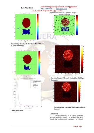
Simulation Results
Side scan sonar Images
close image
10 20 30 40 50 60 70
10
20
30
40
50
60
70
Bot-hat image
10 20 30 40 50 60 70
10
20
30
40
50
60
70

126 | P a g e
Segmentation result of a synthetic image
Probability Density of the Three Pixel Classes
(Good Conditions)
Snake Algorithm:
Conclusion
Image processing is a rapidly growing
area of computer science. Its growth has been
fueled by technological advances in digital
x
y
Morphological clustering image
10 20 30 40 50 60
10
20
30
40
50
60
1
2
3
x
y
Segmentation of Synthetic image
10 20 30 40 50 60
10
20
30
40
50
60
1
2
3
0 10 20 30 40 50 60
0
0.02
0.04
0.06
0.08
0.1
0.12
0.14
0.16
0.18
Normalized historgram and estimated mixture
pixel intensity value
probability
Nomalized histogram
Sum of pdf
Shadow
Background
Target
10 20 30 40 50 60 70
10
20
30
40
50
60
70
5
10
15
20
25
30
35
40
45
50
10 20 30 40 50 60 70
10
20
30
40
50
60
70
5
10
15
20
25
30
35
40
45
50
x
y
Clustering and segmentation of Synthetic image
10 20 30 40 50 60
10
20
30
40
50
60
1
2
3
Iteration Result: Polygon 8 Nodes (Bad Highlight
Contrast)
EM Algorithm
Iteration Result: Polygon 4 Nodes (Bad Highlight
Contrast)

127 | P a g e
imaging, computer processors and mass storage
devices. Fields which traditionally used analog
imaging are now switching to digital systems, for
their flexibility and affordability. Important
examples are medicine, film and video production,
photography, remote sensing, and security
monitoring.
Nowadays, image segmentation represents a task of
growing importance in many different fields. This
technique is finding broad applications in
underwater acoustics, space born remote sensing,
medical imaging systems, non-distractive material
analysis, as well as spoken language
processing[14].
This paper concludes that it is to explore
the potential growth areas of using these two
algorithms in side scan imagery. Evaluating and
comparing their performances for both synthetic
and real sonar images using the software simulation
tool MATLAB.
References
[1] R. Adams and L. Bischof, “Seeded region
growing,” IEEE Trans. Pattern Anal.
Machine Intell., vol. 6, June 1994.
[2] A. C. Bovic, M. Clark, and W. S. Geisler,
“Multichannel texture analysis using
localized spatial filters,” IEEE Trans.
Pattern Anal. Machine Intell., vol. 12, pp.
55–73, Jan. 1990.
[3] J. M. H. Du Buf, “Gabor phase in texture
discrimination,” Signal Process., vol. 21,
pp. 221–240, 1990.
[4] J. M. H. Du Buf and P. Heitkämper,
“Texture features based on Gabor phase,”
Signal Process., vol. 23, pp. 225–244,
1991.
[5] J. Canny, “Computational approach to
edge detection,” IEEE Trans. Pattern
Anal. Machine Intell., vol. 8, pp. 679–698,
Nov. 1986.
[6] L. D. Cohen, “On active contour models
and balloons,” CVGIP: Image
Understand., vol. 53, pp. 211–218, Mar.
1991.
[7] J. G. Daugman and C. J. Downing,
“Demodulation, predictive coding, and
spatial vision,” J. Opt. Soc. Amer. A, vol.
12, pp. 641–660, Apr. 1995.
[8] R. Deriche, “Optimal edge detection using
recursive filtering,” in Proc. IEEE Int.
Conf. Computer Vision, 1987, pp. 501–
505.
[9] D. Dunn, W. E. Higgins, and J. Wakeley,
“Texture segmentation using 2-D Gabor
elementary functions,” IEEE Trans.
Pattern Anal. Machine Intell., vol. 16, pp.
130–149, Feb. 1994.
[10] T. Meier and K. Ngan, “Automatic
segmentation of moving objects for video
object plane generation,” IEEE Trans.
Circuits Syst. Video Technol., vol. 8, pp.
525–538, 1998.
[11] D. Wang, “Unsupervised video
segmentation based on watersheds and
temporal tracking,” IEEE Trans. Circuits
Syst. Video Technol., vol. 8, pp. 539–546,
1998.
[12] C. Gu and M. Lee, “Semiautomatic
segmentation and tracking of semantic
video objects,” IEEE Trans. Circuits Syst.
Video Technol., vol. 8, pp. 572–584,
1998.
[13] M. Kass, A. Witkin, and D. Terzopoulos,
“Snakes: Active contour models,” Int. J.
Comput. Vis., vol. 1, pp. 321–331, 1988.
[14] F. Leymarie and M. Levine, “Tracking
deformable objects in the plane using an
active contour model,” IEEE Trans.
Pattern Anal. Machine Intell.,vol. 15, pp.
617–633, 1993.

W33123127

More Related Content

What's hot

Viewers also liked

Similar to W33123127

Recently uploaded

W33123127