This study investigates the sensitivity of support vector machine (SVM) classification to various training features for remote sensing image classification, specifically using QuickBird images. The research highlights that the choice of spectral and textural features affects classification accuracy, with findings indicating that not all additional features improve performance. Overall, the effectiveness and robustness of SVM in classifying high spatial resolution remote sensing images are validated.
![TELKOMNIKA Indonesian Journal of Electrical Engineering
Vol.12, No.1, January 2014, pp. 286 ~ 291
DOI: http://dx.doi.org/10.11591/telkomnika.v12i1.3969 286
Received June 23, 2013; Revised August 17, 2013; Accepted September 16, 2013
Sensitivity of Support Vector Machine Classification
to Various Training Features
Nanhai Yang, Shuang Li*, Jingwen Liu, FulingBian
International School of Software, Wuhan University
# 37 Luoyu Road, Wuhan, China, 430079, Fax: +86-27-68778221
*corresponding author, e-mail: lishuang129@gmail.com
Abstract
Remote sensing image classification is one of the most important techniques in image
interpretation, which can be used for environmental monitoring, evaluation and prediction. Many algorithms
have been developed for image classification in the literature. Support vector machine (SVM) is a kind of
supervised classification that has been widely used recently. The classification accuracy produced by SVM
may show variation depending on the choice of training features. In this paper, SVM was used for land
cover classification using Quickbird images. Spectral and textural features were extracted for the
classification and the results were analyzed thoroughly. Results showed that the number of features
employed in SVM was not the more the better. Different features are suitable for different type of land
cover extraction. This study verifies the effectiveness and robustness of SVM in the classification of high
spatial resolution remote sensing images.
Keywords: Remote sensing, image classification, support vector machine, feature extraction
Copyright © 2014 Institute of Advanced Engineering and Science. All rights reserved.
1. Introduction
High spatial resolution remote sensing images have played an important role in
mapping, urban planning, defense and military, land use and surveys, and many other areas [1-
3]. As the improvement of spatial resolution, single land cover shows a lot of different spectral
value, which increasing the probability of misclassification. The similar spectral characteristics of
different land covers often lead to confusing in classification, such as shadows and water
bodies, meadows and trees, are often mixed in spectral value. Thus, it is hard to obtain high
classification accuracy when only the spectral information is used. Compared with the traditional
classification methods, Support Vector Machine (SVM) possesses the merits of learning with
small samples, high anti-noise performance, etc. Moreover, SVM also has the advantages of
high learning and promotion efficiency. Therefore, SVM classification showed good performance
in remote sensing image information extraction [4-6].
In this study, SVM was used for land cover classification of Wuhan district in China
using Quickbird images. Various spectral and textural features were extracted for SVM
classification process and classification performances were analyzed thoroughly. It should be
pointed out that the selection of features has an effect on the performance of SVM.
Determination of their optimum combinations is regarded as critical for the success of
classification.
2. Support Vector Machine Algorithm
Support vector machine (SVM) is supervised heuristic algorithm based on statistical
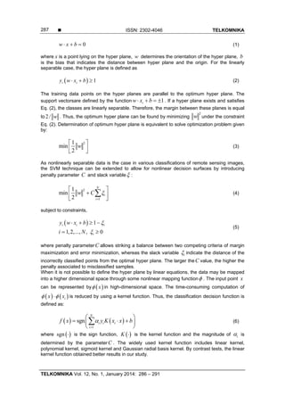
learning theory [7]. The aim of SVM for classification is to determine a hyper plane that optimally
separates two classes. An optimum hyper plane is determined using training data sets and is
verified using test data sets.
Assume data set 1 1, ,..., , ,..., , , 1, 1i i N N ix y x y x y y , where N is the
number of samples, ix is the training sample, iy is the class label of ix . Optimum hyper plane
is used to maximize the margin between classes. The hyper plane is defined as](https://image.slidesharecdn.com/35telkomnikaj6-171212074118/85/Sensitivity-of-Support-Vector-Machine-Classification-to-Various-Training-Features-1-320.jpg)
![TELKOMNIKA Indonesian Journal of Electrical Engineering
Vol.12, No.1, January 2014, pp. 286 ~ 291
DOI: http://dx.doi.org/10.11591/telkomnika.v12i1.3969 286
Received June 23, 2013; Revised August 17, 2013; Accepted September 16, 2013
Sensitivity of Support Vector Machine Classification
to Various Training Features
Nanhai Yang, Shuang Li*, Jingwen Liu, FulingBian
International School of Software, Wuhan University
# 37 Luoyu Road, Wuhan, China, 430079, Fax: +86-27-68778221
*corresponding author, e-mail: lishuang129@gmail.com
Abstract
Remote sensing image classification is one of the most important techniques in image
interpretation, which can be used for environmental monitoring, evaluation and prediction. Many algorithms
have been developed for image classification in the literature. Support vector machine (SVM) is a kind of
supervised classification that has been widely used recently. The classification accuracy produced by SVM
may show variation depending on the choice of training features. In this paper, SVM was used for land
cover classification using Quickbird images. Spectral and textural features were extracted for the
classification and the results were analyzed thoroughly. Results showed that the number of features
employed in SVM was not the more the better. Different features are suitable for different type of land
cover extraction. This study verifies the effectiveness and robustness of SVM in the classification of high
spatial resolution remote sensing images.
Keywords: Remote sensing, image classification, support vector machine, feature extraction
Copyright © 2014 Institute of Advanced Engineering and Science. All rights reserved.
1. Introduction
High spatial resolution remote sensing images have played an important role in
mapping, urban planning, defense and military, land use and surveys, and many other areas [1-
3]. As the improvement of spatial resolution, single land cover shows a lot of different spectral
value, which increasing the probability of misclassification. The similar spectral characteristics of
different land covers often lead to confusing in classification, such as shadows and water
bodies, meadows and trees, are often mixed in spectral value. Thus, it is hard to obtain high
classification accuracy when only the spectral information is used. Compared with the traditional
classification methods, Support Vector Machine (SVM) possesses the merits of learning with
small samples, high anti-noise performance, etc. Moreover, SVM also has the advantages of
high learning and promotion efficiency. Therefore, SVM classification showed good performance
in remote sensing image information extraction [4-6].
In this study, SVM was used for land cover classification of Wuhan district in China
using Quickbird images. Various spectral and textural features were extracted for SVM
classification process and classification performances were analyzed thoroughly. It should be
pointed out that the selection of features has an effect on the performance of SVM.
Determination of their optimum combinations is regarded as critical for the success of
classification.
2. Support Vector Machine Algorithm
Support vector machine (SVM) is supervised heuristic algorithm based on statistical
learning theory [7]. The aim of SVM for classification is to determine a hyper plane that optimally
separates two classes. An optimum hyper plane is determined using training data sets and is
verified using test data sets.
Assume data set 1 1, ,..., , ,..., , , 1, 1i i N N ix y x y x y y , where N is the
number of samples, ix is the training sample, iy is the class label of ix . Optimum hyper plane
is used to maximize the margin between classes. The hyper plane is defined as](https://image.slidesharecdn.com/35telkomnikaj6-171212074118/75/Sensitivity-of-Support-Vector-Machine-Classification-to-Various-Training-Features-1-2048.jpg)
![ISSN: 2302-4046
Sensitivity of Support Vector Machine Classification to Various Training Features (Shuang Li)
288
3. Spectral and Textural Feature Extractions
Many algorithms have been developed for image classification using SVM. Several
factors (e.g. training features, kernel functions, window sizes) have significant impacts on the
classification performance, which should be considered carefully by the analyst. The selection of
appropriate training features depends on the knowledge of land cover types present in the
image by geographers. Thus, training features selection play an important role in the
classification accuracy [8].
3.1. Spectral Feature Extraction
The widely used spectral feature is mean value and the metric derived from spectral
value, i.e. Normalized Difference Vegetation Index (NDVI), Ratio Index (RI), Soil Adjusted
Vegetation Index (SAVI), Normalized Difference Water Index (NDWI). The metric is described in
Table 1.
Table 1. The spectral features used in the study
Metric Equation Description
NDVI R e
R e
N I R d
N I R d
B a n d B a n d
B a n d B a n d
It is used to extract vegetation, i.e. grassland.
RI R e d
N I R
B a n d
B a n d
It is used to extract high density vegetation, i.e. trees.
SAVI R e
R e
1N I R d
N I R d
B a n d B a n d L
B a n d B a n d L
It is used to extract soil with low vegetation cover.
NDWI
G reen N IR
G reen N IR
B and B and
B and B and
It is used to extract water from land covers.
3.2. Textural Features Extraction
The Gray Lever Co-occurrence Matrix (GLCM) is proposed by Haralick in 1970s, which
is an important technique to analyze image texture. The GLCM is based on the second order
combination of probability density function, by calculating the correlation between two points in
the estimated images [9,10]. The texture features are derived from GLCM, i.e. Angular Second
Moment (ASM), Contrast, Entropy and Correlation. Let ,G i j be the element in GLCM and
the size of the matrix be *k k , the metric are described in Table 2.
Table 2. The textural features used in the study
Metric Equation Description
ASM
2
1 1
,
k k
i j
G i j
It denotes the image gray uniformity and texture
coarseness.
Contrast
1
2
| |
0
,
k
i j n
i
n G i j
It reflects the texture clarity.
Entropy
1 1
, l g ( , )
k k
i j
G i j G i j
It measures the amount of information contained in
the image.
Correlation
1 1
1 1 1 1
22
1 1
22
1 1
* ,
, , ,
,
,
k k
i j
i j i j
k k k k
i j
i j i j
k k
i i
i j
k k
j j
i j
i j G i j U U
S S
U i G i j U j G i j
S G i j i U
S G i j j U
It describes the periodicity of texture element in a
certain positional relationship.
4. Experimental Results and Analyze
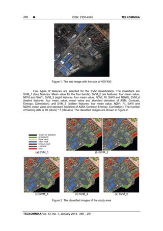
The test image is from Quickbird sensor, with the spectral band ranges from 450nm to
900 nm. The image size is 400*400, which covers water (W), grassland (GL), bare land (BL),
blue roof (BlR), brown roof (BrR), cement surface (CS) and trees (T). The original image is
shown in Figure 1.](https://image.slidesharecdn.com/35telkomnikaj6-171212074118/85/Sensitivity-of-Support-Vector-Machine-Classification-to-Various-Training-Features-3-320.jpg)
![ ISSN: 2302-4046 TELKOMNIKA
TELKOMNIKA Vol. 12, No. 1, January 2014: 286 – 291
291
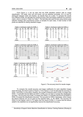
5. Conclusion
Classification of remote sensing images is an important application for image
interpretation. Support vector machine (SVM) have been recently used for many classification
problems. Although it is reported that SVM produce more accurate classification results than the
conventional methods, the selection of optimum training features is one of the most important
issues that affect their performance. In this study, five types of features are used in the
classifiers. From the experiments, several important conclusions can be drawn. Firstly, the
number of features is not the more the better for the classification accuracy, i.e. SVM_3 and
SVM_5. Secondly, the RI and NDWI features perform better than the texture features, including
ASM, Entropy, Contrast and Correlation. This conclusions made here are based on the limited
tests. More comprehensive tests will be conducted in the future.
Acknowledgement
This research was supported by a grant from 973 porject in China (Grant #
2012CB719901)
References
[1] Foody GM, Mathur A. A relative evaluation of multiclass image classification by support vector
machines. IEEE Transactions on Geoscience and Remote Sensing. 2004; 42: 1335-1343.
[2] Han F, Li H, Wen C, Zhao W. A New Incremental Support Vector Machine Algorithm. TELKOMNIKA
Indonesian Journal of Electrical Engineering. 2012; 10: 1171-1178.
[3] Yu Y, Zhou L. Acoustic Emission Signal Classification based on Support Vector Machine.
TELKOMNIKA Indonesian Journal of Electrical Engineering. 2012; 10: 1027-1032.
[4] Shao Y, Lunetta RS. Comparison of support vector machine, neural network, and CART algorithms for
the land-cover classification using limited training data points. ISPRS Journal of Photogrammetry and
Remote Sensing. 2012; 70: 78-87.
[5] Otukei J, Blaschke T. Land cover change assessment using decision trees, support vector machines
and maximum likelihood classification algorithms. International Journal of Applied Earth Observation
and Geoinformation. 2010; 12: S27-S31.
[6] Mountrakis G, Im J, Ogole C. Support vector machines in remote sensing: A review. ISPRS Journal of
Photogrammetry and Remote Sensing. 2011; 66: 247-259.
[7] Vapnik VN. An overview of statistical learning theory. IEEE Transactions on Neural Networks. 1999;
10: 988-999.
[8] Kavzoglu T, Colkesen I. A kernel functions analysis for support vector machines for land cover
classification. International Journal of Applied Earth Observation and Geoinformation. 2009; 11: 352-
359.
[9] Haralick RM, Shanmugam K, Dinstein IH. Textural features for image classification. IEEE
Transactions on Systems, Man and Cybernetics. 1973; 610-621.
[10] Dell'Acqua F, Gamba P. Texture-based characterization of urban environments on satellite SAR
images. IEEE Transactions on Geoscience and Remote Sensing. 2003; 41: 153-159.](https://image.slidesharecdn.com/35telkomnikaj6-171212074118/85/Sensitivity-of-Support-Vector-Machine-Classification-to-Various-Training-Features-6-320.jpg)