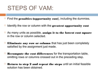
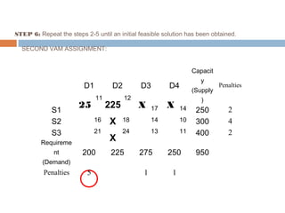
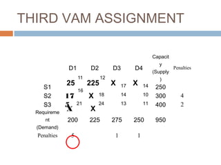
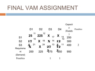
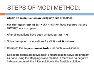
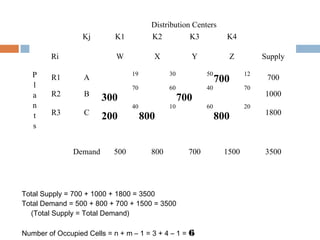
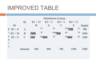
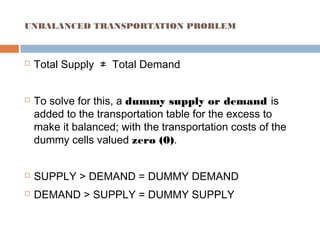
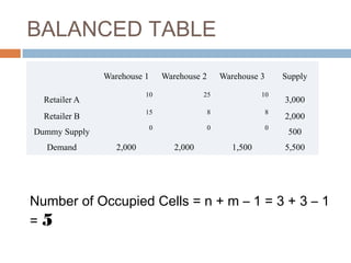
VAM AND MODI
METHODIn Solving Transportation Problems
BY: MANIEGO, Karlo & RIVERA,
Ethel Bianca
TRANSPORTATION MODEL
 Linear programming dealing with the issue of
shipping commodities from multiple sources to
multiple destinations.
 Objective: To determine the shipping schedule
that minimizes the total shipping cost while
satisfying supply and demand constraints.
 A comparative tool in business decision-making.
TRANSPORTATION MODEL
 Main applications:
 Location decisions;
 Production planning;
 Capacity planning; and
 Transshipment
 Major Assumptions:
 Items are homogeneous;
 Shipping cost per unit is the same; and
 Only one route is used from place of shipment to the
destination
TRANSPORTATION PROBLEM
 The following must be known before using a method to
find a low-cost solution:
 Capacity Requirements of the sources (Supply) and of the
destinations (Demand)
 An estimation of the costs of transport per unit
 Number of occupied cells/squares in the table, computed
in formula of n + m – 1, where n is the number of sources
(rows) and m is number of destinations (columns)
TRANSPORTATION TABLE
WAREHOU
SE 1
WAREHOU
SE 2
WAREHOU
SE 3
SUPPLY
PLANT 1 2 4 6 300
PLANT 2 8 6 4 200
PLANT 3 2 4 6 100
DEMAND 100 200 300
DESTINATIONS
SOURCES
TRANSPORTATION COST
PER UNIT
CAPACITYOF
SOURCES
REQUIREMENTS OF
DESTINATIONS
OCCUPIED CELLS = n + m – 1 = 3 + 3 – 1 = 5 CELLS
VOGEL’S APPROXIMATION METHOD (VAM)
 Solution obtained is either optimal or near
to the optimal solution.
 Considers the costs associated with each
route alternative.
STEPS OF VAM:
 Find the penalties (opportunity cost), including the dummies.
 Identify the row or column with the greatest opportunity cost
 As many units as possible, assign it to the lowest cost square
in the row or column selected.
 Eliminate any row or column that has just been completely
satisfied by the assignment just made.
 Recompute the cost differences for the transportation table,
omitting rows or columns crossed out in the preceding step.
 Return to step 2 and repeat the steps until an initial feasible
solution has been obtained.
ILLUSTRATION
 ABC Company has 3 production facilities
S1, S2 and S3 with production capacity of 250,
300 and 400 units per week of a product,
respectively. These units are to be shipped to
4 warehouses D1, D2, D3 and D4 with
requirement of 200, 225, 275 and 250 units per week,
respectively. The transportation costs (in
peso) per unit between factories to
warehouses are given in the table.
Total Supply = 250 + 300 + 400 = 950
Total Demand = 200 + 225 + 275 + 250 = 950
(Total Supply = Total Demand)
Number of Occupied Cells = n + m – 1 = 3 + 4 – 1 = 6
Warehouses
D1 D2 D3 D4
Capacit
y
(Supply)
Pro
duc
tion
Fac
iliti
es
S1 11 12 17 14 250
S2 16 18 14 10 300
S3
21 24 13 11
400
Requireme
nt
(Demand)
200 225 275 250 950
STEP 1: Find the penalties (opportunity cost),
including the dummies, of each row and column.
STEP 2: Identify the row or column with the
greatest opportunity cost
D1 D2 D3 D4
Capacit
y
(Supply
)
Penalties
S1 11 12 17 14 250 1
S2 16 18 14 10 300 4
S3 21 24 13 11 400 2
Requireme
nt
(Demand)
200 225 275 250 950
Penalties 5 6 1 1
PENALTY/OPPORTUNITY COST is the difference between the
two lowest unit shipping costs
STEP 3: Assign as many units as possible to the lowest cost square in the row or column selected.
STEP 4: Eliminate any row or column that has just been completely satisfied by the assignment just made.
D1 D2 D3 D4
Capacit
y
(Supply
)
Penalties
S1 11 17 14 250 1
S2 16 18 14 10 300 4
S3 21 24 13 11 400 2
Requireme
nt
(Demand)
200 225 275 250 950
Penalties 5 6 1 1
22
5
12
X
X
STEP 5: Recompute the cost differences for the transportation table,
omitting rows or columns crossed out in the preceding step.
D1 D2 D3 D4
Capacit
y
(Supply
)
Penalties
S1 11 17 14 250 2
S2 16 18 14 10 300 4
S3 21 24 13 11 400 2
Requireme
nt
(Demand)
200 225 275 250 950
Penalties 5 1 1
225
12
X
X
STEP 6: Repeat the steps 2-5 until an initial feasible solution has been obtained.
SECOND VAM ASSIGNMENT:
D1 D2 D3 D4
Capacit
y
(Supply
)
Penalties
S1 17 14 250 2
S2 16 18 14 10 300 4
S3 21 24 13 11 400 2
Requireme
nt
(Demand)
200 225 275 250 950
Penalties 5 1 1
225
12
X
X
25 XX
11
THIRD VAM ASSIGNMENT
D1 D2 D3 D4
Capacit
y
(Supply
)
Penalties
S1 17 14 250
S2 18 14 10 300 4
S3 21 24 13 11 400 2
Requireme
nt
(Demand)
200 225 275 250 950
Penalties 5 1 1
225
12
X
X
25 XX
11
17
5
16
X
FOURTH VAM ASSIGNMENT
D1 D2 D3 D4
Capacit
y
(Supply
)
Penalties
S1 17 14 250
S2 18 14 300 4
S3 21 24 13 11 400 2
Requireme
nt
(Demand)
200 225 275 250 950
Penalties 1 1
225
12
X
X
25 XX
11
17
5
16
X
10
12
5
X
FINAL VAM ASSIGNMENT
D1 D2 D3 D4
Capacit
y
(Supply
)
Penalties
S1 17 14 250
S2 18 14 300
S3 21 24 13 11 400 2
Requireme
nt
(Demand)
200 225 275 250 950
Penalties 1 1
225
12
X
X
25 XX
11
17
5
16
X
10
12
5
X
27
5
12
5
INITIAL FEASIBLE VAM SOLUTION
D1 D2 D3 D4
Capacit
y
(Supply
)
S1 17 14 250
S2 18 14 300
S3 21 24 13 11 400
Requireme
nt
(Demand)
200 225 275 250 950
225
12
25
11
17
5
16 10
12
5
27
5
12
5
Total Transportation
Cost:
25 units x 11 = 275
225 units x 12 =
2,700
175 units x 16 =
2,800
125 units x 10 =
1,250
275 units x 13 =
3,575
125 units x 11 =
1,375
MODIFIED DISTRIBUTION (MODI) METHOD
 Computing improvement indices quickly
for each unused square without drawing all of
the closed paths.
 The optimality test of the initial feasible
solution
STEPS OF MODI METHOD:
 Obtain an initial solution using any rule or method.
 Set the equations of Ri + Kj = Cij for those squares that are
currently used or occupied.
 After all equations have been written, set R1 = 0
 Solve the system of equations for all R and K values
 Compute the improvement index for each unused square
 Select the largest negative index and proceed to solve the problem
as done using the stepping-stone method. If there are no negative
indices computed, the Initial solution is the feasible solution.
ILLUSTRATION:
 Using the initial VAM solution obtained in the
previous example:
Kj K1 K2 K3 K4
Ri D1 D2 D3 D4 Supply
R1 S1
25
11
225
12 17 14
250
R2 S2
175
16 18 14
125
10
300
R3 S3
21 24
275
13
125
11
400
Demand 200 225 275 250 950
Let:
Ri = value assigned
to row i
Kj = value assigned
to column j
Cij = cost in square
ij (cost of shipping
from source i to
destination j)
STEP 1: Set the equations of Ri + Kj = Cij for those squares that are
currently used or occupied.
 R1 + K1 = 11
 R1 + K2 = 12
 R2 + K1 = 16
 R2 + K4 = 10
 R3 + K3 = 13
 R3 + K4 = 11
Kj K1 K2 K3 K4
Ri D1 D2 D3 D4 Supply
R1 S1
25
11
225
12 17 14
250
R2 S2
175
16 18 14
125
10
300
R3 S3
21 24
275
13
125
11
400
Demand 200 225 275 250 950
STEP 2: After all equations have been written, set R1 = 0
STEP 3: Solve the system of equations for all R and K values
 1. R1 + K1 = 11
0 + K1 = 11K1 = 11
 2. R1 + K2 = 12
0 + K2 = 12 K2 = 12
 
 3. R2 + K1 = 16
R2 + 11 = 16 R2 = 5
 4. R2 + K4 = 10
5 + K4 = 10 K4 = 5
 5. R3 + K4 = 11
R3 + 5 = 11 R3 = 6
 
 6. R3 + K3 = 13
6 + K3 = 13 K3 = 7
IMPROVED TABLE
Kj K1 = 11 K2 = 12 K3 = 7 K4 = 5
Ri D1 D2 D3 D4 Supply
R1 = 0 S1
25
11
225
12 17 14
250
R2 = 5 S2
175
16 18 14
125
10
300
R3 = 6 S3
21 24
275
13
125
11
400
Demand 200 225 275 250 950
STEP 4: Compute the improvement index for each unused square
STEP 5: Select the largest negative index and proceed to solve the problem as done using the stepping-stone method.
 Improvement index formula (Iij) = Cij - Ri – Kj
 S1-D3 index = 17 – R1 – K3 = 17 – 0 – 7 = 10
 S1-D4 index = 14 – R1 – K4 = 14 – 0 – 5 = 9
 S2-D2 index = 18 – R2 – K2 = 18 – 5 – 12 = 1
 S2-D3 index = 14 – R2 – K3 = 14 – 5 – 7 = 2
 S3-D1 index = 21 – R3 – K1 = 21 – 6 – 11 = 4
 S3-D2 index = 24 – R3 – K2 = 24 – 6 – 12 = 6
Since there is no negative index computed, it means that using
the MODI method, the VAM solution is the optimal solution of
ABC Company.
ANOTHER ILLUSTRATION
 A certain company manufactures a certain
product in its three plants, namely Plant A, B,
and C. The plants’ capacities are 700, 1000, and 1800
respectively. The company needs to meet the
demand of its four distribution centers W,
X, Y, and Z with 500, 800, 700, 1500 units respectively.
The transportation cost per unit is provided on
the table. An initial feasible solution is obtained
by Matrix Minimum method as follows:
P
l
a
n
t
s
Distribution Centers
Kj K1 K2 K3 K4
Ri W X Y Z Supply
R1 A
19 30 50
700
12
700
R2 B
300
70 60
700
40 70
1000
R3 C
200
40
800
10 60
800
20
1800
Demand 500 800 700 1500 3500
Total Supply = 700 + 1000 + 1800 = 3500
Total Demand = 500 + 800 + 700 + 1500 = 3500
(Total Supply = Total Demand)
Number of Occupied Cells = n + m – 1 = 3 + 4 – 1 = 6
SOLUTIONS:
 R1 + K4 = 12
 R2 + K1 = 70
 R2 + K3 = 40
 R3 + K1 = 40
 R3 + K2 = 10
 R3 + K4 = 20
 1. R1 + K4 = 12
0 + K4 = 12
K4 = 12
 2. R3 + K4 = 20
R3 + 12 = 20
R3 = 8
 
 3. R3 + K1 = 40
8 + K1 = 40
K1 = 32
 4. R3 + K2 = 10
8 + K2 = 10
K2 = 2
 5. R2 + K1 = 70
R2 + 32 = 70
R2 = 38
 6. R2 + K3 = 40
38 + K3 = 40
K3 = 2
IMPROVED TABLE
P
l
a
n
t
s
Distribution Centers
Kj K1 = 32 K2 = 2 K3 = 2 K4 = 12
Ri W X Y Z Supply
R1 = 0 A 19 30 50
700 12
700
R2 = 38 B 300 70 60
700 40 70
1000
R3 = 8 C 200 40800 10 60800 20 1800
Demand 500 800 700 1500 3500
STEP 5: Select the largest negative index and proceed to solve the problem as
done using the stepping-stone method.
 The Improvement Indices (Iij) are computed as follows:
A-W index = 19 – R1 – K1 = 19 – 0 – 32 = -13
A-X index = 30 – R1 – K2 = 30 – 0 – 2 = 28
A-Y index = 50 – R1 – K3 = 50 – 0 – 2 = 48
B-X index = 30 – R2 – K2 = 60 – 38 – 2 = 20
B-Z index = 60 – R2 – K4 = 60 – 38 – 12 = 10
C-Y index = 60 – R3 – K3 = 60 – 8 – 2 = 50
STEPPING STONE METHOD
 Beginning at the square with the best improvement index, trace a closed path
back to the original square via squares that are currently being used or occupied.
 Beginning with a plus (+) sign at the unused square, place alternate minus (-)
signs and plus signs on each corner square of the closed path just traced.
 Select the smallest quantity found in those squares containing minus signs.
Add that number to all squares on the closed path with plus signs; subtract the
number from all squares assigned minus signs.
 Compute new improvement indices for this new solution using the MODI
method.
STEP 1: Trace a closed path back to the original square
STEP 2: Place alternate plus signs and minus signs on the squares of the traced path
P
l
a
n
t
s
Distribution Centers
W X Y Z Supply
A 19 30 50
700 12
700
B 300 70 60
700 40 70
1000
C 200 40800 10 60800 20 1800
Demand 500 800 700 1500 3500
-
+
+
-
STEP 3: Select the smallest quantity found in those squares
containing minus signs.
Add that number to all squares on the closed path with plus signs;
subtract the number from all squares assigned minus signs.
P
l
a
n
t
s
Distribution Centers
W X Y Z Supply
A 19 30 50
700 12
700
B 300 70 60
700 40 70
1000
C 200 40800 10 60800 20 1800
Demand 500 800 700 1500 3500
-
+
+
-
200
200
200200
NEW MODI SOLUTION
Pla
nts
Distribution Centers
Kj K1 K2 K3 K4
Ri W X Y Z Supply
R1 A
200
19 30 50
500
12
700
R2 B
300
70 60
700
40 70
1000
R3 C
40
800
10 60
1000
20
1800
Demand 500 800 700 1500 3500
SOLUTIONS:
 R1 + K1 = 19
 R1 + K4 = 12
 R2 + K1 = 70
 R2 + K3 = 40
 R3 + K2 = 10
 R3 + K4 = 20
 1. R1 + K4 = 12
0 + K4 = 12 K4 = 12
 2. R1 + K1 = 19
0 + K1 = 19
K1 = 19
 3. R2 + K1 = 70
R2 + 19 = 70
R2 = 51
 4. R2 + K3 = 40
51 + K3 = 40
K3 = -11
 5. R3 + K4 = 20
R3 + 12 = 20
R3 = 8
 6. R3 + K2 = 10
8 + K2 = 10
K2 = 2
IMPROVED NEW MODI SOLUTION
Pla
nts
Distribution Centers
Kj K1 = 19 K2 = 2 K3 = -11 K4 = 12
Ri W X Y Z Supply
R1 = 0 A
200
19 30 50
500
12
700
R2 = 51 B
300
70 60
700
40 70
1000
R3 = 8 C
40
800
10 60
1000
20
1800
Demand 500 800 700 1500 3500
 The Improvement Indices (Iij) are computed as follows:
 A-X index = 30 – R1 – K2 = 30 – 0 – 2 = 28
 A-Y index = 50 – R1 – K3 = 50 – 0 – (-11) = 61
 B-X index = 30 – R2 – K2 = 60 – 51 – 2 = 7
 B-Z index = 70 – R2 – K4 = 70 – 51 – 12 = 7
 C-W index = 40 – R3 – K1 = 40 – 8 – 19 = 13
 C-Y index = 60 – R3 – K3 = 60 – 8 – (-11) = 63
 Since there are no more negative indices computed, the optimal solution of
the company is obtained.
TRANSPORTATION COST
 200 units x 19 = 3,800
 500 units x 12 = 6,000
 300 units x 70 = 21,000
 700 units x 40 = 28,000
 800 units x 10 = 8,000
 1000 units x 20 = 20,000
 Total 86,800
UNBALANCED TRANSPORTATION PROBLEM
 Total Supply ≠ Total Demand
 To solve for this, a dummy supply or demand is
added to the transportation table for the excess to
make it balanced; with the transportation costs of the
dummy cells valued zero (0).
 SUPPLY > DEMAND = DUMMY DEMAND
 DEMAND > SUPPLY = DUMMY SUPPLY
ILLUSTRATION
Warehouse 1 Warehouse 2 Warehouse 3 Supply
Retailer A
10 25 10
3,000
Retailer B
15 8 8
2,000
Demand 2,000 2,000 1,500
Total Supply = 3000 + 2000 = 5000
Total Demand = 2000+ 2000+ 1000 = 5500
(Total Demand > Total Supply = 500 UNITS)
BALANCED TABLE
Warehouse 1 Warehouse 2 Warehouse 3 Supply
Retailer A
10 25 10
3,000
Retailer B
15 8 8
2,000
Dummy Supply
0 0 0
500
Demand 2,000 2,000 1,500 5,500
Number of Occupied Cells = n + m – 1 = 3 + 3 – 1
= 5
OBTAINING INITIAL VAM SOLUTION
FIRST VAM ASSIGNMENT
Warehouse
1
Warehouse
2
Warehouse
3
Supply Penalties
Retailer A
10 25 10
3000 0
Retailer B
15 8 8
2000 0
Dummy
Supply
0 0
500 0
Demand 2000 2000 1500 5500
Penalties 10 8 6
0
50
0
X X
OBTAINING INITIAL VAM SOLUTION
SECOND VAM ASSIGNMENT
Warehouse
1
Warehouse
2
Warehouse
3
Supply Penalties
Retailer A
10 25 10
3000 0
Retailer B
15 8 8
2000 0
Dummy
Supply
0 0
500
Demand 2000 2000 1500 5500
Penalties 5 17 8
0
50
0
X X
2000
X
OBTAINING INITIAL VAM SOLUTION
FINAL VAM ASSIGNMENT
Warehouse
1
Warehouse
2
Warehouse
3
Supply Penalties
Retailer A
10 25 10
3000 0
Retailer B
15 8 8
2000 0
Dummy
Supply
0 0
500
Demand 2000 2000 1500 5500
Penalties 5 8
0
50
0
X X
2000
X 15001500
XX
INITIAL FEASIBLE VAM SOLUTION
Warehouse
1
Warehouse
2
Warehouse
3
Supply Penalties
Retailer A
10 25 10
3000 0
Retailer B
15 8 8
2000 0
Dummy
Supply
0 0
500
Demand 2000 2000 1500 5500
Penalties 5 8
0
50
0
0
2000
15001500
SOLUTIONS USING MODI METHOD:
 R1 + K1 = 10
 R1 + K3 = 10
 R2 + K2 = 8
 R3 + K1 = 0
 R3 + K2 = 0
 1. R1 + K1 = 10
0 + K1 = 10
K1 = 10
 2. R1 + K3 = 10
0 + K3 = 10
K3 = 10
 
 3. R3 + K1 = 0
R3 + 10 = 0 R3 = -10
 
 4. R3 + K2 = 0
-10 + K2 = 0 K2 = 10
 5. R2 + K2 = 8
R2 + 10 = 8 R2 = -2
Since there is no negative index computed, it means that using the
MODI method, the VAM solution is the optimal solution of the company.
 The Improvement Indices (Iij) are computed as follows:
 
 RA-W2 index = 25 – R1 – K2 = 25 – 0 – 10 = 15
 RB-W1 index = 15 – R2 – K1 = 15 – (-2) – 10 = 7
 RB-W3 index = 8 – R2 – K3 = 8 – (-2) – 10 = 0
 RD-W3 index = 0 – R3 – K3 = 0 – (-10) – 10 = 0
TRANSPORTATION COST
 1500 units x 10 = 15,000
 2000 units x 8 = 16,000
 500 units x 0 = 0
 Total 46,000

VAM and MODI Method in Solving Transportation Problems

  • 1.
    VAM AND MODI METHODInSolving Transportation Problems BY: MANIEGO, Karlo & RIVERA, Ethel Bianca
  • 2.
    TRANSPORTATION MODEL  Linearprogramming dealing with the issue of shipping commodities from multiple sources to multiple destinations.  Objective: To determine the shipping schedule that minimizes the total shipping cost while satisfying supply and demand constraints.  A comparative tool in business decision-making.
  • 3.
    TRANSPORTATION MODEL  Mainapplications:  Location decisions;  Production planning;  Capacity planning; and  Transshipment  Major Assumptions:  Items are homogeneous;  Shipping cost per unit is the same; and  Only one route is used from place of shipment to the destination
  • 4.
    TRANSPORTATION PROBLEM  Thefollowing must be known before using a method to find a low-cost solution:  Capacity Requirements of the sources (Supply) and of the destinations (Demand)  An estimation of the costs of transport per unit  Number of occupied cells/squares in the table, computed in formula of n + m – 1, where n is the number of sources (rows) and m is number of destinations (columns)
  • 5.
    TRANSPORTATION TABLE WAREHOU SE 1 WAREHOU SE2 WAREHOU SE 3 SUPPLY PLANT 1 2 4 6 300 PLANT 2 8 6 4 200 PLANT 3 2 4 6 100 DEMAND 100 200 300 DESTINATIONS SOURCES TRANSPORTATION COST PER UNIT CAPACITYOF SOURCES REQUIREMENTS OF DESTINATIONS OCCUPIED CELLS = n + m – 1 = 3 + 3 – 1 = 5 CELLS
  • 6.
    VOGEL’S APPROXIMATION METHOD(VAM)  Solution obtained is either optimal or near to the optimal solution.  Considers the costs associated with each route alternative.
  • 7.
    STEPS OF VAM: Find the penalties (opportunity cost), including the dummies.  Identify the row or column with the greatest opportunity cost  As many units as possible, assign it to the lowest cost square in the row or column selected.  Eliminate any row or column that has just been completely satisfied by the assignment just made.  Recompute the cost differences for the transportation table, omitting rows or columns crossed out in the preceding step.  Return to step 2 and repeat the steps until an initial feasible solution has been obtained.
  • 8.
    ILLUSTRATION  ABC Companyhas 3 production facilities S1, S2 and S3 with production capacity of 250, 300 and 400 units per week of a product, respectively. These units are to be shipped to 4 warehouses D1, D2, D3 and D4 with requirement of 200, 225, 275 and 250 units per week, respectively. The transportation costs (in peso) per unit between factories to warehouses are given in the table.
  • 9.
    Total Supply =250 + 300 + 400 = 950 Total Demand = 200 + 225 + 275 + 250 = 950 (Total Supply = Total Demand) Number of Occupied Cells = n + m – 1 = 3 + 4 – 1 = 6 Warehouses D1 D2 D3 D4 Capacit y (Supply) Pro duc tion Fac iliti es S1 11 12 17 14 250 S2 16 18 14 10 300 S3 21 24 13 11 400 Requireme nt (Demand) 200 225 275 250 950
  • 10.
    STEP 1: Findthe penalties (opportunity cost), including the dummies, of each row and column. STEP 2: Identify the row or column with the greatest opportunity cost D1 D2 D3 D4 Capacit y (Supply ) Penalties S1 11 12 17 14 250 1 S2 16 18 14 10 300 4 S3 21 24 13 11 400 2 Requireme nt (Demand) 200 225 275 250 950 Penalties 5 6 1 1 PENALTY/OPPORTUNITY COST is the difference between the two lowest unit shipping costs
  • 11.
    STEP 3: Assignas many units as possible to the lowest cost square in the row or column selected. STEP 4: Eliminate any row or column that has just been completely satisfied by the assignment just made. D1 D2 D3 D4 Capacit y (Supply ) Penalties S1 11 17 14 250 1 S2 16 18 14 10 300 4 S3 21 24 13 11 400 2 Requireme nt (Demand) 200 225 275 250 950 Penalties 5 6 1 1 22 5 12 X X
  • 12.
    STEP 5: Recomputethe cost differences for the transportation table, omitting rows or columns crossed out in the preceding step. D1 D2 D3 D4 Capacit y (Supply ) Penalties S1 11 17 14 250 2 S2 16 18 14 10 300 4 S3 21 24 13 11 400 2 Requireme nt (Demand) 200 225 275 250 950 Penalties 5 1 1 225 12 X X
  • 13.
    STEP 6: Repeatthe steps 2-5 until an initial feasible solution has been obtained. SECOND VAM ASSIGNMENT: D1 D2 D3 D4 Capacit y (Supply ) Penalties S1 17 14 250 2 S2 16 18 14 10 300 4 S3 21 24 13 11 400 2 Requireme nt (Demand) 200 225 275 250 950 Penalties 5 1 1 225 12 X X 25 XX 11
  • 14.
    THIRD VAM ASSIGNMENT D1D2 D3 D4 Capacit y (Supply ) Penalties S1 17 14 250 S2 18 14 10 300 4 S3 21 24 13 11 400 2 Requireme nt (Demand) 200 225 275 250 950 Penalties 5 1 1 225 12 X X 25 XX 11 17 5 16 X
  • 15.
    FOURTH VAM ASSIGNMENT D1D2 D3 D4 Capacit y (Supply ) Penalties S1 17 14 250 S2 18 14 300 4 S3 21 24 13 11 400 2 Requireme nt (Demand) 200 225 275 250 950 Penalties 1 1 225 12 X X 25 XX 11 17 5 16 X 10 12 5 X
  • 16.
    FINAL VAM ASSIGNMENT D1D2 D3 D4 Capacit y (Supply ) Penalties S1 17 14 250 S2 18 14 300 S3 21 24 13 11 400 2 Requireme nt (Demand) 200 225 275 250 950 Penalties 1 1 225 12 X X 25 XX 11 17 5 16 X 10 12 5 X 27 5 12 5
  • 17.
    INITIAL FEASIBLE VAMSOLUTION D1 D2 D3 D4 Capacit y (Supply ) S1 17 14 250 S2 18 14 300 S3 21 24 13 11 400 Requireme nt (Demand) 200 225 275 250 950 225 12 25 11 17 5 16 10 12 5 27 5 12 5 Total Transportation Cost: 25 units x 11 = 275 225 units x 12 = 2,700 175 units x 16 = 2,800 125 units x 10 = 1,250 275 units x 13 = 3,575 125 units x 11 = 1,375
  • 18.
    MODIFIED DISTRIBUTION (MODI)METHOD  Computing improvement indices quickly for each unused square without drawing all of the closed paths.  The optimality test of the initial feasible solution
  • 19.
    STEPS OF MODIMETHOD:  Obtain an initial solution using any rule or method.  Set the equations of Ri + Kj = Cij for those squares that are currently used or occupied.  After all equations have been written, set R1 = 0  Solve the system of equations for all R and K values  Compute the improvement index for each unused square  Select the largest negative index and proceed to solve the problem as done using the stepping-stone method. If there are no negative indices computed, the Initial solution is the feasible solution.
  • 20.
    ILLUSTRATION:  Using theinitial VAM solution obtained in the previous example: Kj K1 K2 K3 K4 Ri D1 D2 D3 D4 Supply R1 S1 25 11 225 12 17 14 250 R2 S2 175 16 18 14 125 10 300 R3 S3 21 24 275 13 125 11 400 Demand 200 225 275 250 950 Let: Ri = value assigned to row i Kj = value assigned to column j Cij = cost in square ij (cost of shipping from source i to destination j)
  • 21.
    STEP 1: Setthe equations of Ri + Kj = Cij for those squares that are currently used or occupied.  R1 + K1 = 11  R1 + K2 = 12  R2 + K1 = 16  R2 + K4 = 10  R3 + K3 = 13  R3 + K4 = 11 Kj K1 K2 K3 K4 Ri D1 D2 D3 D4 Supply R1 S1 25 11 225 12 17 14 250 R2 S2 175 16 18 14 125 10 300 R3 S3 21 24 275 13 125 11 400 Demand 200 225 275 250 950
  • 22.
    STEP 2: Afterall equations have been written, set R1 = 0 STEP 3: Solve the system of equations for all R and K values  1. R1 + K1 = 11 0 + K1 = 11K1 = 11  2. R1 + K2 = 12 0 + K2 = 12 K2 = 12    3. R2 + K1 = 16 R2 + 11 = 16 R2 = 5  4. R2 + K4 = 10 5 + K4 = 10 K4 = 5  5. R3 + K4 = 11 R3 + 5 = 11 R3 = 6    6. R3 + K3 = 13 6 + K3 = 13 K3 = 7
  • 23.
    IMPROVED TABLE Kj K1= 11 K2 = 12 K3 = 7 K4 = 5 Ri D1 D2 D3 D4 Supply R1 = 0 S1 25 11 225 12 17 14 250 R2 = 5 S2 175 16 18 14 125 10 300 R3 = 6 S3 21 24 275 13 125 11 400 Demand 200 225 275 250 950
  • 24.
    STEP 4: Computethe improvement index for each unused square STEP 5: Select the largest negative index and proceed to solve the problem as done using the stepping-stone method.  Improvement index formula (Iij) = Cij - Ri – Kj  S1-D3 index = 17 – R1 – K3 = 17 – 0 – 7 = 10  S1-D4 index = 14 – R1 – K4 = 14 – 0 – 5 = 9  S2-D2 index = 18 – R2 – K2 = 18 – 5 – 12 = 1  S2-D3 index = 14 – R2 – K3 = 14 – 5 – 7 = 2  S3-D1 index = 21 – R3 – K1 = 21 – 6 – 11 = 4  S3-D2 index = 24 – R3 – K2 = 24 – 6 – 12 = 6 Since there is no negative index computed, it means that using the MODI method, the VAM solution is the optimal solution of ABC Company.
  • 25.
    ANOTHER ILLUSTRATION  Acertain company manufactures a certain product in its three plants, namely Plant A, B, and C. The plants’ capacities are 700, 1000, and 1800 respectively. The company needs to meet the demand of its four distribution centers W, X, Y, and Z with 500, 800, 700, 1500 units respectively. The transportation cost per unit is provided on the table. An initial feasible solution is obtained by Matrix Minimum method as follows:
  • 26.
    P l a n t s Distribution Centers Kj K1K2 K3 K4 Ri W X Y Z Supply R1 A 19 30 50 700 12 700 R2 B 300 70 60 700 40 70 1000 R3 C 200 40 800 10 60 800 20 1800 Demand 500 800 700 1500 3500 Total Supply = 700 + 1000 + 1800 = 3500 Total Demand = 500 + 800 + 700 + 1500 = 3500 (Total Supply = Total Demand) Number of Occupied Cells = n + m – 1 = 3 + 4 – 1 = 6
  • 27.
    SOLUTIONS:  R1 +K4 = 12  R2 + K1 = 70  R2 + K3 = 40  R3 + K1 = 40  R3 + K2 = 10  R3 + K4 = 20  1. R1 + K4 = 12 0 + K4 = 12 K4 = 12  2. R3 + K4 = 20 R3 + 12 = 20 R3 = 8    3. R3 + K1 = 40 8 + K1 = 40 K1 = 32  4. R3 + K2 = 10 8 + K2 = 10 K2 = 2  5. R2 + K1 = 70 R2 + 32 = 70 R2 = 38  6. R2 + K3 = 40 38 + K3 = 40 K3 = 2
  • 28.
    IMPROVED TABLE P l a n t s Distribution Centers KjK1 = 32 K2 = 2 K3 = 2 K4 = 12 Ri W X Y Z Supply R1 = 0 A 19 30 50 700 12 700 R2 = 38 B 300 70 60 700 40 70 1000 R3 = 8 C 200 40800 10 60800 20 1800 Demand 500 800 700 1500 3500
  • 29.
    STEP 5: Selectthe largest negative index and proceed to solve the problem as done using the stepping-stone method.  The Improvement Indices (Iij) are computed as follows: A-W index = 19 – R1 – K1 = 19 – 0 – 32 = -13 A-X index = 30 – R1 – K2 = 30 – 0 – 2 = 28 A-Y index = 50 – R1 – K3 = 50 – 0 – 2 = 48 B-X index = 30 – R2 – K2 = 60 – 38 – 2 = 20 B-Z index = 60 – R2 – K4 = 60 – 38 – 12 = 10 C-Y index = 60 – R3 – K3 = 60 – 8 – 2 = 50
  • 30.
    STEPPING STONE METHOD Beginning at the square with the best improvement index, trace a closed path back to the original square via squares that are currently being used or occupied.  Beginning with a plus (+) sign at the unused square, place alternate minus (-) signs and plus signs on each corner square of the closed path just traced.  Select the smallest quantity found in those squares containing minus signs. Add that number to all squares on the closed path with plus signs; subtract the number from all squares assigned minus signs.  Compute new improvement indices for this new solution using the MODI method.
  • 31.
    STEP 1: Tracea closed path back to the original square STEP 2: Place alternate plus signs and minus signs on the squares of the traced path P l a n t s Distribution Centers W X Y Z Supply A 19 30 50 700 12 700 B 300 70 60 700 40 70 1000 C 200 40800 10 60800 20 1800 Demand 500 800 700 1500 3500 - + + -
  • 32.
    STEP 3: Selectthe smallest quantity found in those squares containing minus signs. Add that number to all squares on the closed path with plus signs; subtract the number from all squares assigned minus signs. P l a n t s Distribution Centers W X Y Z Supply A 19 30 50 700 12 700 B 300 70 60 700 40 70 1000 C 200 40800 10 60800 20 1800 Demand 500 800 700 1500 3500 - + + - 200 200 200200
  • 33.
    NEW MODI SOLUTION Pla nts DistributionCenters Kj K1 K2 K3 K4 Ri W X Y Z Supply R1 A 200 19 30 50 500 12 700 R2 B 300 70 60 700 40 70 1000 R3 C 40 800 10 60 1000 20 1800 Demand 500 800 700 1500 3500
  • 34.
    SOLUTIONS:  R1 +K1 = 19  R1 + K4 = 12  R2 + K1 = 70  R2 + K3 = 40  R3 + K2 = 10  R3 + K4 = 20  1. R1 + K4 = 12 0 + K4 = 12 K4 = 12  2. R1 + K1 = 19 0 + K1 = 19 K1 = 19  3. R2 + K1 = 70 R2 + 19 = 70 R2 = 51  4. R2 + K3 = 40 51 + K3 = 40 K3 = -11  5. R3 + K4 = 20 R3 + 12 = 20 R3 = 8  6. R3 + K2 = 10 8 + K2 = 10 K2 = 2
  • 35.
    IMPROVED NEW MODISOLUTION Pla nts Distribution Centers Kj K1 = 19 K2 = 2 K3 = -11 K4 = 12 Ri W X Y Z Supply R1 = 0 A 200 19 30 50 500 12 700 R2 = 51 B 300 70 60 700 40 70 1000 R3 = 8 C 40 800 10 60 1000 20 1800 Demand 500 800 700 1500 3500
  • 36.
     The ImprovementIndices (Iij) are computed as follows:  A-X index = 30 – R1 – K2 = 30 – 0 – 2 = 28  A-Y index = 50 – R1 – K3 = 50 – 0 – (-11) = 61  B-X index = 30 – R2 – K2 = 60 – 51 – 2 = 7  B-Z index = 70 – R2 – K4 = 70 – 51 – 12 = 7  C-W index = 40 – R3 – K1 = 40 – 8 – 19 = 13  C-Y index = 60 – R3 – K3 = 60 – 8 – (-11) = 63  Since there are no more negative indices computed, the optimal solution of the company is obtained.
  • 37.
    TRANSPORTATION COST  200units x 19 = 3,800  500 units x 12 = 6,000  300 units x 70 = 21,000  700 units x 40 = 28,000  800 units x 10 = 8,000  1000 units x 20 = 20,000  Total 86,800
  • 38.
    UNBALANCED TRANSPORTATION PROBLEM Total Supply ≠ Total Demand  To solve for this, a dummy supply or demand is added to the transportation table for the excess to make it balanced; with the transportation costs of the dummy cells valued zero (0).  SUPPLY > DEMAND = DUMMY DEMAND  DEMAND > SUPPLY = DUMMY SUPPLY
  • 39.
    ILLUSTRATION Warehouse 1 Warehouse2 Warehouse 3 Supply Retailer A 10 25 10 3,000 Retailer B 15 8 8 2,000 Demand 2,000 2,000 1,500 Total Supply = 3000 + 2000 = 5000 Total Demand = 2000+ 2000+ 1000 = 5500 (Total Demand > Total Supply = 500 UNITS)
  • 40.
    BALANCED TABLE Warehouse 1Warehouse 2 Warehouse 3 Supply Retailer A 10 25 10 3,000 Retailer B 15 8 8 2,000 Dummy Supply 0 0 0 500 Demand 2,000 2,000 1,500 5,500 Number of Occupied Cells = n + m – 1 = 3 + 3 – 1 = 5
  • 41.
    OBTAINING INITIAL VAMSOLUTION FIRST VAM ASSIGNMENT Warehouse 1 Warehouse 2 Warehouse 3 Supply Penalties Retailer A 10 25 10 3000 0 Retailer B 15 8 8 2000 0 Dummy Supply 0 0 500 0 Demand 2000 2000 1500 5500 Penalties 10 8 6 0 50 0 X X
  • 42.
    OBTAINING INITIAL VAMSOLUTION SECOND VAM ASSIGNMENT Warehouse 1 Warehouse 2 Warehouse 3 Supply Penalties Retailer A 10 25 10 3000 0 Retailer B 15 8 8 2000 0 Dummy Supply 0 0 500 Demand 2000 2000 1500 5500 Penalties 5 17 8 0 50 0 X X 2000 X
  • 43.
    OBTAINING INITIAL VAMSOLUTION FINAL VAM ASSIGNMENT Warehouse 1 Warehouse 2 Warehouse 3 Supply Penalties Retailer A 10 25 10 3000 0 Retailer B 15 8 8 2000 0 Dummy Supply 0 0 500 Demand 2000 2000 1500 5500 Penalties 5 8 0 50 0 X X 2000 X 15001500 XX
  • 44.
    INITIAL FEASIBLE VAMSOLUTION Warehouse 1 Warehouse 2 Warehouse 3 Supply Penalties Retailer A 10 25 10 3000 0 Retailer B 15 8 8 2000 0 Dummy Supply 0 0 500 Demand 2000 2000 1500 5500 Penalties 5 8 0 50 0 0 2000 15001500
  • 45.
    SOLUTIONS USING MODIMETHOD:  R1 + K1 = 10  R1 + K3 = 10  R2 + K2 = 8  R3 + K1 = 0  R3 + K2 = 0  1. R1 + K1 = 10 0 + K1 = 10 K1 = 10  2. R1 + K3 = 10 0 + K3 = 10 K3 = 10    3. R3 + K1 = 0 R3 + 10 = 0 R3 = -10    4. R3 + K2 = 0 -10 + K2 = 0 K2 = 10  5. R2 + K2 = 8 R2 + 10 = 8 R2 = -2
  • 46.
    Since there isno negative index computed, it means that using the MODI method, the VAM solution is the optimal solution of the company.  The Improvement Indices (Iij) are computed as follows:    RA-W2 index = 25 – R1 – K2 = 25 – 0 – 10 = 15  RB-W1 index = 15 – R2 – K1 = 15 – (-2) – 10 = 7  RB-W3 index = 8 – R2 – K3 = 8 – (-2) – 10 = 0  RD-W3 index = 0 – R3 – K3 = 0 – (-10) – 10 = 0
  • 47.
    TRANSPORTATION COST  1500units x 10 = 15,000  1500 units x 10 = 15,000  2000 units x 8 = 16,000  500 units x 0 = 0  Total 46,000