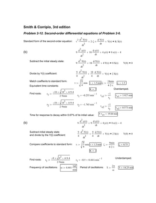
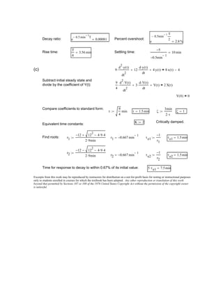
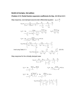
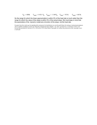
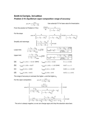
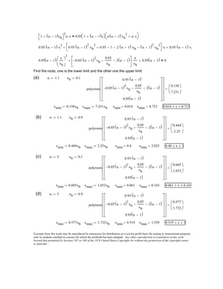
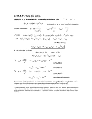
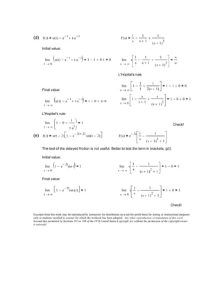
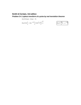
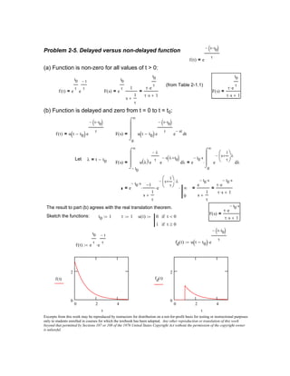
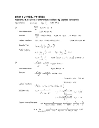
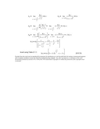
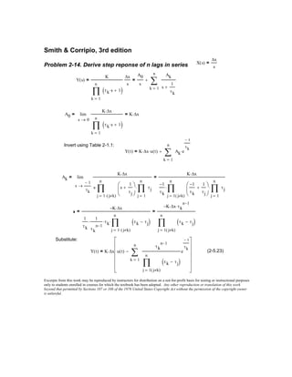
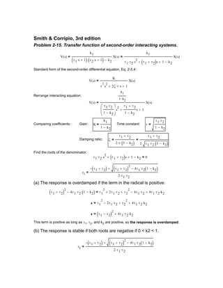
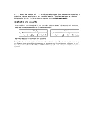
The document derives several Laplace transforms from their definitions using properties like linearity and complex translations. It also checks the initial and final value problems of the derived transforms. Key results derived include: 1) The Laplace transform of functions like t, t^2, e^-at, cos(ωt), and their linear combinations. 2) The use of properties like linearity, complex translations, and L'Hopital's rule to derive transforms. 3) Initial and final value checks of the derived transforms to validate the solutions.

1. F s( )
s
s
2
ω
2
+
=
1
2
1
s i ω⋅−
1
s i ω⋅+
+




=
s i ω⋅− s+ i ω⋅+
2 s i ω⋅−( )⋅ s i ω⋅+( )
=
2 s⋅
2 s
2
ω
2
+( )⋅
=
s
s
2
ω
2
+
=
1
2
1−
s i ω⋅−
e
s i ω⋅−( )t−
∞
0
⋅
1−
s i ω⋅+
e
s i ω⋅+( )t−
∞
0
⋅+





=
1
2 0
∞
te
s i ω⋅−( )t−⌠

⌡
d
0
∞
te
s i ω⋅+( )t−⌠

⌡
d+








=
F s( )
0
∞
tcos ωt⋅ e
st−
⋅
⌠

⌡
d=
0
∞
t
e
i ωt⋅
e
i− ωt⋅
−
2
e
st−
⌠


⌡
d=f t( ) cos ωt⋅=(c)
F s( )
1
s a+
=
F s( )
0
∞
te
at−
e
st−⌠

⌡
d=
0
∞
te
s a+( )t−⌠

⌡
d=
1−
s a+
e
s a+( )t−
∞
0
⋅=
1
s a+
=
where a is constantf t( ) e
at−
=(b)
F s( )
1
s
2
=
F s( )
t−
s
e
st−
∞
0
⋅
1
s 0
∞
te
st−⌠

⌡
d⋅+= 0 0−
1
s
2
e
st−
∞
0
⋅−=
1
s
2
=
v
1−
s
e
st−
=du dt=
dv e
st−
dt=u t=By parts:F s( )
0
∞
tt e
st−
⋅
⌠

⌡
d=f t( ) t=(a)
F s( )
0
∞
tf t( ) e
st−⌠

⌡
d=
Problem 2-1. Derivation of Laplace transforms from its definition
Smith & Corripio, 3rd. edition

2. (d) f t( ) e
at−
coss ωt⋅=
F s( )
0
∞
te
at−
cos ωt⋅ e
st−
⋅
⌠

⌡
d=
0
∞
te
at− e
i ωt⋅
e
i− ωt⋅
+
2
⋅ e
st−
⌠


⌡
d=
1
2 0
∞
te
s a+ i ω⋅+( )t−⌠

⌡
d
0
∞
te
s a+ i ω⋅−( )− t⌠

⌡
d+








=
1
2
1−
s a+ i ω⋅+
e
s a+ i ω⋅+( )t−
∞
0
⋅
1−
s a+ i ω⋅−
e
s a+ i ω⋅−( )t−
∞
0
⋅+





=
1
2
1
s a+ i ω⋅+
1
s a+ i ω⋅−
+




=
s a+ i ω⋅− s+ a+ i ω⋅+
2 s a+ i ω⋅+( ) s a+ i ω⋅−( )
=
2 s a+( )
2 s a+( )
2
ω
2
+


⋅
=
s a+
s a+( )
2
ω
2
+
= F s( )
s a+
s a+( )
2
ω
2
+
=
All the results match results in Table 2-1.1
Excerpts from this work may be reproduced by instructors for distribution on a not-for-profit basis for testing or instructional purposes
only to students enrolled in courses for which the textbook has been adopted. Any other reproduction or translation of this work
beyond that permitted by Sections 107 or 108 of the 1976 United States Copyright Act without the permission of the copyright owner
is unlawful.

3. 1
s
1
s 2+
+ 2
1
s 1+
⋅−=
1
s
1
s 2+
+
2
s 1+
−=
F s( )
1
s
1
s 2+
+
2
s 1+
−=
Used the linearity property.
(d) f t( ) u t( ) e
t−
− t e
t−
⋅+= F s( ) L u t( )( ) L e
t−
( )− L t e
t−
⋅( )+=
1
s
1
s 1+
−
1
s 1+( )
2
+=
F s( )
1
s
1
s 1+
−
1
s 1+( )
2
+=
Used the linearity property.
(e) f t( ) u t 2−( ) 1 e
2− t 2−( )
sin t 2−( )− = Let g t( ) u t( ) 1 e
2− t
sin t⋅−( )= Then f t( ) g t 2−( )=
F s( ) e
2− s
G s( )= e
2− s 1
s
1
s 2+( )
2
1+
−





=
Used the real translation theorem and linearity. F s( ) e
2− s 1
s
1
s 2+( )
2
1+
−





=
Excerpts from this work may be reproduced by instructors for distribution on a not-for-profit basis for testing or instructional purposes
only to students enrolled in courses for which the textbook has been adopted. Any other reproduction or translation of this work
beyond that permitted by Sections 107 or 108 of the 1976 United States Copyright Act without the permission of the copyright owner
is unlawful.
Smith & Corripio, 3rd edition
Problem 2-2. Derive Laplace transforms from the properties and Table 2-1.1
(a) f t( ) u t( ) 2 t⋅+ 3 t
2
⋅+= F s( ) L u t( ) 2 t⋅+ 3 t
2
⋅+( )= L u t( )( ) 2 L t( )⋅+ 3 L t
2
( )⋅+=
1
s
2
1
s
2
⋅+ 3
2!
s
3
⋅+= F s( )
1
s
2
s
2
+
6
s
3
+=
Used the linearity property.
(b) f t( ) e
2− t⋅
u t( ) 2 t⋅+ 3 t
2
⋅+( )= F s( ) L u t( ) 2 t⋅+ 3 t
2
⋅+( )
s 2+
⋅=
1
s
2
s
2
+
6
s
3
+



 s 2+
⋅=
1
s 2+
2
s 2+( )
2
+
6
s 2+( )
3
+=
F s( )
1
s 2+
2
s 2+( )
2
+
6
s 2+( )
3
+=
Used the complex translation theorem.
(c) f t( ) u t( ) e
2− t
+ 2e
t−
−= F s( ) L u t( ) e
2− t
+ 2 e
t−
⋅−( )= L u t( )( ) L e
2− t
( )+ 2 L e
t−
( )⋅−=

4. Must apply L'Hopital's rule:
∞s
1
1
2
2 s 2+( )
+
6
3 s 2+( )
2
+





1=lim
→Final value:
∞t
e
2− t
u t( ) 2 t⋅+ 3t
2
+( ) 0 ∞⋅=lim
→
0s
s
1
s 2+
2
s 2+( )
2
+
6
s 3+( )
2
+





0=lim
→
L'Hopital's rule:
∞t
0
2e
2t
2
2e
2t
+
6t
2e
2t
+




0=lim
→
Check!
(c) f t( ) u t( ) e
2− t
+ 2e
t−
−= F s( )
1
s
1
s 2+
+
2
s 1+
−=
Initial value:
0t
u t( ) e
2− t
+ 2e
t−
−( ) 1 1+ 2−( ) 0+=lim
→ ∞s
s
1
s
1
s 2+
+
2
s 1+
−




∞
∞
=lim
→
L'Hopital's rule:
∞s
1
1
1
+
2
1
−




0=lim
→
Final value:
∞t
u t( ) e
2− t
+ 2e
t−
−( ) 1 0+ 0+= 1=lim
→ 0s
s
1
s
1
s 2+
+
2
s 1+
−




1 0+ 0+= 1=lim
→
Smith & Corripio, 3rd edition
Problem 2-3. Initial and final value check of solutions to Problem 2-2
(a) f t( ) u t( ) 2 t⋅+ 3t
2
+= F s( )
1
s
2
s
2
+
6
s
3
+=
Initial value:
0t
u t( ) 2t+ 3t
2
+( ) 1=lim
→ ∞s
s
1
s
2
s
2
+
6
s
3
+




⋅
∞s
1
2
s
+
6
s
2
+




1=lim
→
=lim
→
Final value:
∞t
u t( ) 2t+ 3t
2
+( ) ∞=lim
→ 0s
1
2
s
+
6
s
2
+




∞=lim
→
Check!
(b) f t( ) e
2− t
u t( ) 2t+ 3t
2
+( )= F s( )
1
s 2+
2
s 2+( )
2
+
6
s 2+( )
3
+=
Initial value:
0t
e
2− t
u t( ) 2t+ 3t
2
+( )lim
→ ∞s
s
1
s 2+
2
s 2+( )
2
+
6
s 2+( )
3
+





∞
∞
=lim
→
1 1 0+ 0+( )= 1=

5. Excerpts from this work may be reproduced by instructors for distribution on a not-for-profit basis for testing or instructional purposes
only to students enrolled in courses for which the textbook has been adopted. Any other reproduction or translation of this work
beyond that permitted by Sections 107 or 108 of the 1976 United States Copyright Act without the permission of the copyright owner
is unlawful.
Check!
0s
s
1
s
1
s 1+( )
2
1+
−





1 0+= 1=lim
→∞t
1 e
2− t
sin t( )⋅−  1=lim
→
Final value:
∞s
s
1
s
1
s 1+( )
2
1+
−





1 0−= 1=lim
→0t
1 e
2− t
sin t⋅−( ) 1=lim
→
Initial value:
The test of the delayed fnction is not useful. Better to test the term in brackets, g(t):
F s( ) e
2− s 1
s
1
s 1+( )
2
1+
−





=f t( ) u t 2−( ) 1 e
2− t 2−( )
sin t 2−( )− =(e)
Check!
∞t
1 0−
1
1 e
t
⋅
+




1=lim
→
L'Hopital's rule:
∞t
u t( ) e
t−
− t e
t−
⋅+( ) 1 0− ∞ 0⋅+=lim
→
0s
1
s
s 1+
−
s
s 1+( )
2
+





1 0− 0+= 1=lim
→
Final value: ∞s
1
1
1
−
1
2 s 1+( )
+





1 1− 0+= 0=lim
→
L'Hopital's rule:
∞s
s
1
s
1
s 1+
−
1
s 1+( )
2
+





∞
∞
=lim
→0t
u t( ) e
t−
− t e
t−
⋅+( ) 1 1− 0 1⋅+= 0=lim
→
Initial value:
F s( )
1
s
1
s 1+
−
1
s 1+( )
2
+=f t( ) u t( ) e
t−
− t e
t−
⋅+=(d)

6. Smith & Corripio, 3rd edition
Problem 2-4. Laplace transform of a pulse by real translation theorem
f t( ) H u t( )⋅ H u t T−( )⋅−=
F s( ) H
1
s
⋅ H e
sT−
⋅
1
s
⋅−= H
1 e
sT−
−
s
⋅= F s( )
H
s
1 e
sT−
−( )=

7. Excerpts from this work may be reproduced by instructors for distribution on a not-for-profit basis for testing or instructional purposes
only to students enrolled in courses for which the textbook has been adopted. Any other reproduction or translation of this work
beyond that permitted by Sections 107 or 108 of the 1976 United States Copyright Act without the permission of the copyright owner
is unlawful.
0 2 4
0
2
fd t( )
t
0 2 4
0
2
f t( )
t
f t( ) e
t0
τ
e
t−
τ
⋅:=
fd t( ) u t t0−( ) e
t t0−( )−
τ
⋅:=
u t( ) 0 t 0<if
1 t 0≥if
:=τ 1:=t0 1:=Sketch the functions:
F s( )
τ e
t0− s⋅
⋅
τ s⋅ 1+
=
The result to part (b) agrees with the real translation theorem.
e
t0− s⋅ 1−
s
1
τ
+
⋅ e
s
1
τ
+





− λ⋅
⋅ ∞
0
⋅=
e
t0− s⋅
s
1
τ
+
=
τ e
t0− s⋅
⋅
τ s⋅ 1+
=
F s( )
t0−
∞
λu λ( )e
λ−
τ
e
s λ t0+( )−
⌠



⌡
d= e
t0− s⋅
0
∞
λe
s
1
τ
+





λ−
⌠



⌡
d⋅=
λ t t0−=Let
F s( )
0
∞
tu t t0−( )e
t t0−( )−
τ
e
st−
⌠



⌡
d=f t( ) u t t0−( )e
t t0−( )−
τ
=
(b) Function is delayed and zero from t = 0 to t = t0:
F s( )
τ e
t0
τ
⋅
τ s⋅ 1+
=F s( ) e
t0
τ 1
s
1
τ
+
=
τ e
t0
τ
⋅
τ s⋅ 1+
=f t( ) e
t0
τ
e
t−
τ
=
(from Table 2-1.1)
(a) Function is non-zero for all values of t > 0:
f t( ) e
t t0−( )−
τ
=
Problem 2-5. Delayed versus non-delayed function

8. Y t( ) 2.5− e
t−
2.5u t( )+= (Table 2-1.1)
(b)
9
d
2
y t( )⋅
dt
2
⋅ 18
d y t( )⋅
dt
⋅+ 4 y t( )+ 8 x t( ) 4−=
Initial steady state: 4 y 0( )⋅ 8 x 0( ) 4−=
Subtract:
9
d
2
Y t( )⋅
dt
2
⋅ 18
d Y t( )⋅
dt
⋅+ 4 Y t( )+ 8 X t( )=
Y t( ) y t( ) y 0( )−= Y 0( ) 0=
X t( ) x t( ) x 0( )−=
Laplace transform:
9s
2
Y s( ) 18s Y s( )⋅+ 4 Y s( )+ 8 X s( )= 8
1
s
⋅=
Solve for Y(s): Y s( )
8
9s
2
18s+ 4+
1
s
=
r1
18− 18
2
4 9⋅ 4⋅−+
2 9⋅
:= r1 0.255−=
r2
18− 18
2
4 9⋅ 4⋅−−
2 9⋅
:= r2 1.745−=
Expand in partial fractions:
Y s( )
8
9 s 0.255+( ) s 1.745+( )s
=
A1
s 0.255+
A2
s 1.745+
+
A3
s
+=
A1
0.255−s
8
9 s 1.745+( )s
8
9 0.255− 1.745+( )⋅ 0.255−( )⋅
= 2.342−=lim
→
=
Smith & Corripio, 3rd edition
Problem 2-6. Solution of differential equations by Laplace transforms
Input function: X t( ) u t( )= X s( )
1
s
= (Table 2-1.1)
(a)
d y t( )⋅
dt
2 y t( )+ 5 x t( ) 3+=
Initial steady state: 2 y 0( ) 5 x 0( )= 3=
Subtract:
d Y t( )⋅
dt
2 Y t( )+ 5 X t( )= Y t( ) y t( ) y 0( )−= X t( ) x t( ) x 0( )−=
Laplace transform: sY s( ) Y 0( )− 2 Y s( )+ 5 X s( )= 5
1
s
⋅= Y 0( ) y 0( ) y 0( )−= 0=
Solve for Y(s):
Y s( )
5
s 2+
1
s
=
A1
s 2+
A2
s
+=
Partial fractions:
A1
2−s
5
s
2.5−=lim
→
= A2
0s
5
s 2+
2.5=lim
→
=
Y s( )
5−
s 1+
5
s
+= Invert:

9. Y 0( ) 0=9
d
2
Y t( )⋅
dt
2
⋅ 12
d Y t( )⋅
dt
⋅+ 4 Y t( )+ 8 X t( )=
Subtract initial steady state:
9
d
2
y t( )⋅
dt
2
⋅ 12
d y t( )⋅
dt
⋅+ 4 y t( )+ 8 x t( ) 4−=(d)
Y t( ) 1− 1.134i+( )e
0.5− 0.441i+( )t
1− 1.134i−( )e
0.5− 0.441i−( )t
+ 2 u t( )+=
Invert using
Table 2-1.1:
Y s( )
1− 1.134i+
s 0.5+ 0.441i−
1− 1.134i−
s 0.5+ 0.441i+
+
2
s
+=
A3
0s
8
9s
2
9s+ 4+
2=lim
→
=A2 1− 1.134i−=
8
9 2 0.441i⋅( ) 0.5− 0.441i+( )
1− 1.134i+=A1
0.5− 0.441i+s
8
9 s 0.5+ 0.441i+( ) s
lim
→
=
A1
s 0.5+ 0.441i−
A2
s 0.5+ 0.441i+
+
A3
s
+=
Y s( )
8
9 s 0.5+ 0.441i−( ) s 0.5+ 0.441+( )s
=Solve for Y(s), expand:
A2
1.745−s
8
9 s 0.255+( )s
8
9 1.745− 0.255+( ) 1.745−( )
= 0.342=lim
→
=
A3
0s
8
9 s 0.255+( ) s 1.745+( )
8
9 0.255( ) 1.745( )
= 2.0=lim
→
=
Y s( )
2.342−
s 0.255+
0.342
s 1.745+
+
2
s
+=
Invert with Table 2-1.1:
Y t( ) 2.342− e
0.255− t
0.342e
1.745− t
+ 2 u t( )+=
(c) 9
d
2
y t( )⋅
dt
2
⋅ 9
d y t( )⋅
dt
⋅+ 4 y t( )+ 8 x t( ) 4−=
Subtract initial steady state:
9
d
2
Y t( )⋅
dt
2
⋅ 9
d Y t( )⋅
dt
⋅+ 4 Y t( )+ 8 X t( )= Y 0( ) 0=
Laplace transform:
9s
2
9s+ 4+( )Y s( ) 8 X s( )= 8
1
s
⋅=
r1
9− 9
2
4 9⋅ 4⋅−+
2 9⋅
:= r2
9− 9
2
4 9⋅ 4⋅−−
2 9⋅
:= r1 0.5− 0.441i+=
Find roots:
r2 0.5− 0.441i−=

10. A2 0.027 0.022i−=
3
2 2 2.598i⋅( ) 1− 2.598i+( ) 1.5− 2.598i+( )
0.027 0.022i+=
A1
1.5− 2.598i+s
3
2 s 1.5+ 2.598i+( ) s 0.5+( )s
0.027 0.022i+=lim
→
=
A1
s 1.5+ 2.598i−
A2
s 1.5+ 2.598i+
+
A3
s 0.5+
+
A4
s
+=
Y s( )
3
2 s 1.5+ 2.598i−( ) s 1.5+ 2.598i+( ) s 0.5+( )s
=Solve for Y(s) and expand:
polyroots
9
21
7
2



















1.5− 2.598i−
1.5− 2.598i+
0.5−






=
Find roots:
2s
3
7s
2
+ 21s+ 9+( )Y s( ) 3 X s( )= 3
1
s
⋅=Laplace transform:
Y 0( ) 0=
2
d
3
Y t( )⋅
dt
3
⋅ 7
d
2
Y t( )⋅
dt
2
⋅+ 21
d Y t( )⋅
dt
⋅+ 9 Y t( )+ 3 X t( )=Subtract initial steady state:
2
d
3
y t( )⋅
dt
3
⋅ 7
d
2
y t( )⋅
dt
2
⋅+ 21
d y t( )⋅
dt
⋅+ 9 y t( )+ 3 x t( )=(e)
Y t( )
4−
3
t 2−




e
0.667− t
2 u t( )+=Invert using Table 2-1.1:
A3
0s
8
9 s 0.667+( )
2
2=lim
→
=
A2
0.667−s
d
ds
8
9s




 0.667−s
8−
9s
2
2−=lim
→
=lim
→
=A1
0.667−s
8
9s
4−
3
=lim
→
=
Y s( )
8
9 s 0.667+( )
2
s
=
A1
s 0.667+( )
2
A2
s 0.667+
+
A3
s
+=Solve for Y(s) and expand:
r2 0.667−=
r1 0.667−=r2
12− 12
2
4 9⋅ 4⋅−−
2 9⋅
:=r1
12− 12
2
4 9⋅ 4⋅−+
2 9⋅
:=
Find roots:
9s
2
12s+ 4+( )Y s( ) 8 X s( )= 8
1
s
⋅=Laplace transform:

11. A3
0.5−s
3
2 s 1.5+ 2.598i−( ) s 1.5+ 2.598i+( )s
0.387−=lim
→
=
3
2 1 2.598i−( ) 1 2.598i+( ) 0.5−( )
0.387−= A4
0s
3
2s
3
7s
2
+ 21s+ 9+
1
3
=lim
→
=
Y s( )
0.027 0.022i+
s 1.5+ 2.598i−
0.027 0.022i−
s 1.5+ 2.598i+
+
0.387−
s 0.5+
+
1
3
1
s
+=
Invert using Table 2-1.1:
Y t( ) 0.027 0.022i+( )e
1.5− 2.598i+( )t
0.027 0.022i−( )e
1.5− 2.598i−( )t
+ 0.387e
0.5− t
−
1
3
u t( )+=
Excerpts from this work may be reproduced by instructors for distribution on a not-for-profit basis for testing or instructional purposes
only to students enrolled in courses for which the textbook has been adopted. Any other reproduction or translation of this work
beyond that permitted by Sections 107 or 108 of the 1976 United States Copyright Act without the permission of the copyright owner
is unlawful.

12. Excerpts from this work may be reproduced by instructors for distribution on a not-for-profit basis for testing or instructional purposes
only to students enrolled in courses for which the textbook has been adopted. Any other reproduction or translation of this work
beyond that permitted by Sections 107 or 108 of the 1976 United States Copyright Act without the permission of the copyright owner
is unlawful.
Y t( ) u t 1−( )
8−
3
t 1−( )⋅ 8−





e
0.667− t 1−( )⋅
⋅ 8 e
0.333− t 1−( )⋅
⋅+





⋅=
Apply the real translation theorem in reverse to this solution:
Y s( )
8−
3
1
s 0.667+( )
2
8
s 0.667+
−
8
s 0.333+
+





e
s−
=
The partial fraction expansion of the undelayed signal is the same:
(Real translation
theorem)
X s( )
e
s−
s
1
3
+
=X t( ) u t 1−( ) e
t 1−( )−
3
=(b) Forcing function:
Y t( )
8−
3
t 8−




e
0.667− t
8e
0.333− t
+=Invert using Table 2-1.1:
Y s( )
8−
3
1
s 0.667+( )
2
8−
s 0.667+
+
8
s 0.333+
+=
A2
0.667−s
d
ds
8
9 s 0.333+( )





 0.667−s
8−
9 s 0.333+( )
2
8−=lim
→
=lim
→
=
A3
0.333−s
8
9 s 0.667+( )
2
8=lim
→
=A1
0.667−s
8
9 s 0.333+( )
8−
3
=lim
→
=
8
9 s 0.667+( )
2
s 0.333+( )
=
A1
s 0.667+( )
2
A2
s 0.667+
+
A3
s 0.333+
+=
Y s( )
8
9s
2
12s+ 4+( ) s
1
3
+




=
X s( )
1
s
1
3
+
=From Table 2-1.1:X t( ) e
t−
3
=(a) Forcing function:
Y 0( ) 0=9
d
2
Y t( )⋅
dt
2
⋅ 12
d Y t( )⋅
dt
⋅+ 4 Y t( )+ 8 X t( )=
Problem 2-7. Solve Problem 2-6(d) with different forcing functions
Smith & Corripio, 3rd edition

13. (Final value theorem)
(b)
9
d
2
y t( )⋅
dt
2
⋅ 18
d y t( )⋅
dt
⋅+ 4 y t( )+ 8 x t( ) 4−=
Subtract initial steady state: 9
d
2
Y t( )⋅
dt
2
⋅ 18
d Y t( )⋅
dt
⋅+ 4 Y t( )+ 8 X t( )= Y 0( ) 0=
Laplace transform and solve for Y(s): Y s( )
8
9s
2
18s+ 4+
X s( )=
Find roots: r1
18− 18
2
4 9⋅ 4⋅−+
2 9⋅ min
:= r2
18− 18
2
4 9⋅ 4⋅−−
2 9⋅ min
:= r1 0.255− min
1−
=
r2 1.745− min
1−
=
Invert using Table 2-1.1: Y t( ) A1 e
0.255− t
⋅ A2 e
1.745− t
⋅+=
+ terms of X(s)
The response is stable and monotonic. The domnant root is: r1 0.255− min
1−
=
Time for the response to decay to 0.67% of its initial value:
5−
r1
19.6 min=
Final steady-state value for unit step input:
0s
s
8
9s
2
18s+ 4+
⋅
1
s
lim
→
2→
(Final value theorem)
Smith & Corripio, 3rd edition
Problem 2-8. Response characteristics of the equations of Problem 2-6
(a)
d y t( )⋅
dt
2 y t( )+ 5 x t( ) 3+=
Initial steady state: 2 y 0( ) 5 x 0( ) 3+=
Subtract:
d Y t( )⋅
dt
2 Y t( )+ 5 X t( )= Y t( ) y t( ) y 0( )−= X t( ) x t( ) x 0( )−=
Laplace transform: s Y s( )⋅ 2 Y s( )+ 5 X s( )= Y 0( ) y 0( ) y 0( )−= 0=
Solve for Y(s): Y s( )
5
s 2+
X s( )=
A1
s 2+
= + terms of X(s)
Invert using Table 2-1.1: Y t( ) A1 e
2− t
⋅= + terms of X(t)
The response is stable and monotonic.The dominant and only root is r 2− min
1−
:=
Time for response to decay to within 0.67% of its initial value:
5−
r
2.5min=
Final steady-state value for unit step input:
0s
s
5
s 2+
⋅
1
s
lim
→
5
2
→ 2.5=

14. Time for oscillations to die:
5−
0.5− min
1−
10 min=
Final steady state value for a unit step imput:
0s
s
8
9s
2
9s+ 4+
⋅
1
s
lim
→
2→
(Final value theorem)
(d) 9
d
2
y t( )⋅
dt
2
⋅ 12
d y t( )⋅
dt
⋅+ 4 y t( )+ 8 x t( ) 4−=
Subtract initial steady state:
9
d
2
Y t( )⋅
dt
2
⋅ 12
d Y t( )⋅
dt
⋅+ 4 Y t( )+ 8 X t( )=
Y 0( ) 0=
Laplace transform and solve for Y(s): Y s( )
8
9s
2
12s+ 4+
X s( )=
Find roots: r1
12− 12
2
4 9⋅ 4⋅−+
2 9⋅ min
:= r2
12− 12
2
4 9⋅ 4⋅−−
2 9⋅ min
:= r1 0.667− min
1−
=
r2 0.667− min
1−
=
Invert using Table 2-1.1: Y t( ) A1 t⋅ A2+( )e
0.667− t
= + terms of X(t)
(c) 9
d
2
y t( )⋅
dt
2
⋅ 9
d y t( )⋅
dt
⋅+ 4 y t( )+ 8 x t( ) 4−=
Subtract initial steady state: 9
d
2
Y t( )⋅
dt
2
⋅ 9
d Y t( )⋅
dt
⋅+ 4 Y t( )+ 8 X t( )= Y 0( ) 0=
Laplace transform and solve for Y(s): Y s( )
8
9s
2
9s+ 4+
X s( )=
Find the roots: r1
9− 9
2
4 9⋅ 4⋅−+
2 9⋅ min
:= r2
9− 9
2
4 9⋅ 4⋅−−
2 9⋅ min
:= r1 0.5− 0.441i+ min
1−
=
r2 0.5− 0.441i− min
1−
=
Invert using Table 2-3.1: Y t( ) D e
0.5− t
⋅ sin 0.441t θ+( )= + terms of X(t)
The response is stable and oscillatory. The dominant roots are r1 and r2.
Period of the oscillations: T
2π
0.441min
1−
:= T 14.25 min=
Decay ratio: e
0.5− min
1−
T
0.00081=

15. Excerpts from this work may be reproduced by instructors for distribution on a not-for-profit basis for testing or instructional purposes
only to students enrolled in courses for which the textbook has been adopted. Any other reproduction or translation of this work
beyond that permitted by Sections 107 or 108 of the 1976 United States Copyright Act without the permission of the copyright owner
is unlawful.
(Final value theorem)
0s
s
3
2s
3
7s
2
+ 21s+ 9+
⋅
1
s
lim
→
1
3
→Final steady state value for a unit step input:
5−
r
2
10 min=Time for response to die out:e
1.5− min
1−
T
0.027=
Decay ratio:
T 2.42 min=T
2π
2.598min
1−
:=The period of the oscillations is:
r
2
0.5− min
1−
=The response is stable and oscillatory. The dominant root is
r
1.5− 2.598i−
1.5− 2.598i+
0.5−






min
1−
=r polyroots
9
21
7
2



















min
1−
:=
Find roots:
Y s( )
3
2s
3
7s
2
+ 21s+ 9+
X s( )=Laplace transform and solve for Y(s):
2
d
3
Y t( )⋅
dt
3
⋅ 7
d
2
Y t( )⋅
dt
2
⋅+ 21
d Y t( )⋅
dt
⋅+ 9 Y t( )+ 3 X t( )=Subtract initial steady state:
2
d
3
y t( )⋅
dt
3
⋅ 7
d
2
y t( )⋅
dt
2
⋅+ 21
d y t( )⋅
dt
⋅+ 9 y t( )+ 3 x t( )=(e)
(Final value theorem)
0s
s
8
9s
2
12s+ 4+
⋅
1
s
lim
→
2→Final steady state value for a unit step input:
5−
r1
7.5min=Time required for the response to decay within 0.67% of its initial value:
r1 0.667− min
1−
=The response is stable and monotonic. The dominant root is

16. Value of k: k
M− g⋅
y0
:= k 1.816
N
m
=
Laplace transform:
M s
2
⋅ Y s( ) k Y s( )⋅+ F s( )=
Solve for Y(s): Y s( )
1
M s
2
⋅ k+
F s( )=
A1
s i
k
M
⋅−
A2
s i
k
M
⋅+
+=
+ terms of F(s)
θ 0:=
D 1:=
Invert using Table 2-3.1: Y t( ) D sin
k
M
t s⋅ θ+





⋅:= + terms of f(t)
The mobile will oscillate forever with a period of T 2π
M
k
⋅:= T 1.043 s=
Smith & Corripio, 3rd edition
Problem 2-9. Second-Order Response: Bird Mobile
-Mg
f(t)
y(t)
-ky(t)
y = 0
Problem data: M 50gm:= y0 27− cm:=
Solution:
Force balance:
M
d v t( )⋅
dt
⋅ M− g⋅ k y t( )⋅− f t( )+=
Velocity:
d y t( )⋅
dt
v t( )=
Initial steady state: 0 M− g⋅ k y0⋅−=
Subtract and substitute:
M
d
2
Y t( )⋅
dt
2
⋅ k− Y t( )⋅ f t( )+=
Y 0( ) 0=

17. 0 2 4
1
0
1
Y t( )
t
To more accurately reflect the motion of the bird mobile, we must add the resistance of the air. If we
assume it to be a force proportional to the velocity:
M
d
2
Y t( )⋅
dt
2
⋅ k− Y t( )⋅ b
d Y t( )⋅
dt
⋅− f t( )+=
With this added term the roots will have a negative real part, causing the oscillations to decay, as
they do in practice:
Y s( )
1
M s
2
⋅ b s⋅+ k+
F s( )= r1
b− b
2
4M k⋅−+
2M
=
b−
2M
i
k
M
b
2
4M
2
−⋅+=
Invert:
b
2
4M k⋅<
Y t( ) D e
b−
2M
t⋅
⋅ sin
k
M
b
2
4M
2
− t θ+






= + terms of f(t)
Excerpts from this work may be reproduced by instructors for distribution on a not-for-profit basis for testing or instructional purposes
only to students enrolled in courses for which the textbook has been adopted. Any other reproduction or translation of this work
beyond that permitted by Sections 107 or 108 of the 1976 United States Copyright Act without the permission of the copyright owner
is unlawful.

18. H 1:=T 1:=τ 1:=KH 1:=Invert using Table 2-1.1, and the real translation theorem:
Y s( ) K H
1
s
1
s
1
τ
+
−





⋅ 1 e
sT−
−( )=
A2
0s
K H⋅
τ s⋅ 1+
K H⋅=lim
→
=A1
1−
τ
s
K H⋅
τ s⋅
K− H⋅=lim
→
=
Y s( )
K
τ s⋅ 1+
H⋅
1 e
sT−
−
s
⋅=
A1
s
1
τ
+
A2
s
+






1 e
sT−
−( )=Substitute:
X s( ) H
1 e
sT−
−
s
⋅=
From Example 2-1.1b:
(b) Pulse of Fig. 2-1.1b
0 2 4
0
0.5
1
Y t( )
t
Y t( )
K
τ
e
t−
τ
:=
Invert using Table 2-1.1:
Y s( )
K
τ s⋅ 1+
=
X s( ) 1=From Table 2-1.1:X t( ) δ t( )=(a) Unit impulse:
Y s( )
K
τ s⋅ 1+
X s( )=Laplace transform and solve for Y(s):
Y 0( ) 0=τ
d Y t( )⋅
dt
⋅ Y t( )+ K X t( )⋅=
Problem 2-10. Responses of general first-order differential equation
Smith & Corripio, 3rd edition

19. Y t( ) KH u t( ) e
t−
τ
− u t T−( ) 1 e
t T−( )−
τ
−





⋅−





⋅:=
X t( ) H u t( ) u t T−( )−( )⋅:=
0 2 4
0
0.5
1
Y t( )
X t( )
t
Excerpts from this work may be reproduced by instructors for distribution on a not-for-profit basis for testing or instructional purposes
only to students enrolled in courses for which the textbook has been adopted. Any other reproduction or translation of this work
beyond that permitted by Sections 107 or 108 of the 1976 United States Copyright Act without the permission of the copyright owner
is unlawful.

20. Excerpts from this work may be reproduced by instructors for distribution on a not-for-profit basis for testing or instructional purposes
only to students enrolled in courses for which the textbook has been adopted. Any other reproduction or translation of this work
beyond that permitted by Sections 107 or 108 of the 1976 United States Copyright Act without the permission of the copyright owner
is unlawful.
The tank is an integrating process because its ouput, the level, is the time integral of its input, the
inlet flow.
0 5 10
0
5
10
h t( )
t
f(t)
h(t)
A 1:=
h t( )
1
A
t:=Invert using Table 2-1.1:H s( )
1
A
1
s
2
=Substitute:
(Table 2-1.1)F s( )
1
s
=f t( ) u t( )=Response to a unit step in flow:
H s( )
F s( )
1
A s⋅
=Transfer function of the tank:
H s( )
1
A s⋅
F s( )=Laplace transform and solve for H(s):
h 0( ) 0=A
d h t( )⋅
dt
⋅ f t( )=
Problem 2-11. Response of an integrating process
Smith & Corripio, 3rd edition

21. r2 1.745− min
1−
=
τe2
1−
r2
:=
τe2 0.573 min=
5 τe1⋅ 19.64 min=
Time for response to decay within 0.67% of its initial value:
(b) 9
d
2
y t( )⋅
dt
2
⋅ 9
d y t( )⋅
dt
⋅+ 4 y t( )+ 8 x t( ) 4−=
Subtract initial steady state
and divide by the Y(t) coefficient:
9
4
d
2
Y t( )⋅
dt
2
⋅
9
4
d Y t( )⋅
dt
⋅+ Y t( )+ 2 X t( )= Y 0( ) 0=
Compare coefficients to standard form: τ
9
4
min:= τ 1.5min= ζ
9min
4 2⋅ τ⋅
:= ζ 0.75=
K 2:=
Underdamped.
Find roots: r1
9− 9
2
4 9⋅ 4⋅−+
2 9⋅ min
:= r1 0.5− 0.441i+ min
1−
=
Frequency of oscillations: ω 0.441
rad
min
:= Period of oscillations: T
2π
ω
:= T 14.25 min=
Smith & Corripio, 3rd edition
Problem 2-12. Second-order differeential equations of Problem 2-6.
Standard form of the second-order equation: τ
2 d
2
Y t( )⋅
dt
2
⋅ 2 ζ⋅ τ⋅
d Y t( )⋅
dt
⋅+ Y t( )+ K X t( )⋅=
(b) 9
d
2
y t( )⋅
dt
2
⋅ 18
d y t( )⋅
dt
⋅+ 4 y t( )+ 8 x t( ) 4−=
Subtract the initial steady state:
9
d
2
Y t( )⋅
dt
2
⋅ 18
d Y t( )⋅
dt
⋅+ 4 Y t( )+ 8 X t( )= Y 0( ) 0=
Divide by Y(t) coefficient:
9
4
d
2
Y t( )⋅
dt
2
⋅
18
4
d Y t( )⋅
dt
⋅+ Y t( )+ 2 X t( )=
Match coeffients to standard form:
τ
9
4
min:= τ 1.5min= ζ
18min
4 2⋅ τ⋅
:= ζ 1.5=
Equivalent time constants:
K 2:= Overdamped.
Find roots: r1
18− 18
2
4 9⋅ 4⋅−+
2 9⋅ min
:=
r1 0.255− min
1−
= τe1
1−
r1
:= τe1 3.927 min=
r2
18− 18
2
4 9⋅ 4⋅−−
2 9⋅ min
:=

22. ζ 1=
K 2:= Critically damped.
Equivalent time constants:
Find roots: r1
12− 12
2
4 9⋅ 4⋅−+
2 9⋅ min
:= r1 0.667− min
1−
= τe1
1−
r1
:= τe1 1.5min=
r2
12− 12
2
4 9⋅ 4⋅−−
2 9⋅ min
:=
r2 0.667− min
1−
= τe2
1−
r2
:= τe2 1.5min=
Time for response to decay to within 0.67% of its initial value: 5 τe1⋅ 7.5min=
Excerpts from this work may be reproduced by instructors for distribution on a not-for-profit basis for testing or instructional purposes
only to students enrolled in courses for which the textbook has been adopted. Any other reproduction or translation of this work
beyond that permitted by Sections 107 or 108 of the 1976 United States Copyright Act without the permission of the copyright owner
is unlawful.
Decay ratio: e
0.5− min
1−
T
0.00081= Percent overshoot:
e
0.5− min
1− T
2
2.8%=
Rise time:
T
4
3.56 min= Settling time:
5−
0.5− min
1−
10 min=
(c) 9
d
2
y t( )⋅
dt
2
⋅ 12
d y t( )⋅
dt
⋅+ 4 y t( )+ 8 x t( ) 4−=
Subtract initial steady state and
divide by the coefficient of Y(t):
9
4
d
2
Y t( )⋅
dt
2
⋅ 3
d Y t( )⋅
dt
⋅+ Y t( )+ 2 X t( )=
Y 0( ) 0=
Compare coefficients to standard form:
τ
9
4
min:= τ 1.5min= ζ
3min
2 τ⋅
:=

23. Y s( ) K ∆x
1−
τ
1
s
1
τ
+




2
1
s
1
τ
+






−
1
s
+







⋅=
A2
1−
τ
s
d
ds
K ∆x⋅
τ
2
s




 1−
τ
s
K− ∆x⋅
τ
2
s
2
K− ∆x⋅=lim
→
=lim
→
=
A3
0s
K ∆x⋅
τ s⋅ 1+( )2
K ∆x⋅=lim
→
=A1
1−
τ
s
K ∆x⋅
τ
2
s
K− ∆x⋅
τ
=lim
→
=
Y s( )
K
τ s⋅ 1+( )2
∆x
s
=
A1
s
1
τ
+




2
A2
s
1
τ
+
+
A3
s
+=
Step response for the critically damped case:
Y t( ) K ∆x u t( )
τe1
τe1 τe2−
e
t−
τe1
−
τe2
τe2 τe1−
e
t−
τe2
−








⋅=
(2-5.10)Invert using Table 2-1.1:
Y s( ) K ∆x
τe1−
τe1 τe2−
1
s
1
τe1
+
τe2
τe2 τe1−
1
s
1
τe2
+
−
1
s
+








⋅=
A3
0s
K ∆x⋅
τe1 s⋅ 1+( ) τe2 s⋅ 1+( )
K ∆x⋅=lim
→
=
A2
K− ∆x⋅ τe2⋅
τe2 τe1−
=A1
1−
τe1
s
K ∆x⋅
τe1 τe2⋅ s
1
τe2
+




⋅ s
K− ∆x⋅ τe1⋅
τe1 τe2−
=lim
→
=
Y s( )
K
τe1 s⋅ 1+( ) τe2 s⋅ 1+( )
∆x
s
=
A1
s
1
τe1
+
A2
s
1
τe2
+
+
A3
s
+=
X s( )
∆x
s
=Step response, over-damped second-order differential equation:
Problem 2-13. Partial fraction expansion coefficients for Eqs. 2-5.10 to 2-5.13
Smith & Corripio, 3rd edition

24. Y s( )
K
τ s⋅ 1+( )2
r
s
2
=
A1
s
1
τ
+




2
A2
s
1
τ
+
+
A3
s
2
+
A4
s
+=
Ramp response for critically damped case:
Y t( ) K r
τe1
2
τe1 τe2−
e
t−
τe1
τe2
2
τe2 τe1−
e
t−
τe2
+ t+ τe1 τe2+( )−










⋅=
(2-5.12)
Invert using Table 2-1.1:
Y s( ) K r
τe1
2
τe1 τe2−
1
s
1
τe1
+
τe2
2
τe2 τe1−
1
s
1
τe2
+
+
1
s
2
+
τe1 τe2+
s
−








⋅=
K r τe1− τe2−( )⋅=
A4
0s
d
ds
K r⋅
τe1 s⋅ 1+( ) τe2 s⋅ 1+( )⋅






⋅
0s
K r⋅
τe1− τe2 s⋅ 1+( )⋅ τe2 τe1 s⋅ 1+( )⋅−
τe1 s⋅ 1+( )
2
τe2 s⋅ 1+( )
2
⋅lim
→
=lim
→
=
A3
0s
K r⋅
τe1 s⋅ 1+( ) τe2 s⋅ 1+( )⋅
K r⋅=lim
→
=
A2
K r⋅ τe2
2
⋅
τe2 τe1−
=A1
1−
τe1
s
K r⋅
τe1 τe2⋅ s
1
τe2
+




⋅ s
2
⋅
K r⋅ τe1
2
⋅
τe1 τe2−
=lim
→
=
Y s( )
K
τe1 s⋅ 1+( ) τe2 s⋅ 1+( )⋅
r
s
2
=
A1
s
1
τe1
+
A2
s
1
τe2
+
+
A3
s
2
+
A4
s
+=
X s( )
r
s
2
=Ramp response for the over-damped case:
Y t( ) K ∆x u t( )
t
τ
1+




e
t−
τ
−








⋅=
(2-5.11)
Invert using Table 2-1.1:

25. A1
1−
τ
s
K r⋅
τ
2
s
2
K r⋅=lim
→
= A3
0s
K r⋅
τ s⋅ 1+( )2
K r⋅=lim
→
=
A2
1−
τ
s
d
ds
K r⋅
τ
2
s
2




 1−
τ
s
2−
K r⋅
τ
2
s
3
⋅ 2 K⋅ r⋅ τ⋅=lim
→
=lim
→
=
A4
0s
d
ds
K r⋅
τ s⋅ 1+( )2





 0s
2−
K r⋅ τ⋅
τ s⋅ 1+( )3
⋅ 2− K⋅ r⋅ τ⋅=lim
→
=lim
→
=
Y s( ) K r
1
s
1
τ
+




2
2 τ⋅
s
1
τ
+
+
1
s
2
+
2 τ⋅
s
−










⋅=
Invert using Table 2-1.1:
Y t( ) K r⋅ t 2 τ⋅+( )e
t−
τ
t+ 2 τ⋅−





⋅= (2-5.13)
Excerpts from this work may be reproduced by instructors for distribution on a not-for-profit basis for testing or instructional purposes
only to students enrolled in courses for which the textbook has been adopted. Any other reproduction or translation of this work
beyond that permitted by Sections 107 or 108 of the 1976 United States Copyright Act without the permission of the copyright owner
is unlawful.

26. Smith & Corripio, 3rd edition
X s( )
∆x
s
=
Problem 2-14. Derive step reponse of n lags in series
Y s( )
K
1
n
k
τk s⋅ 1+( )∏
=
∆x
s
=
A0
s
1
n
k
Ak
s
1
τk
+
∑
=
+=
A0
0s
K ∆x⋅
1
n
k
τk s⋅ 1+( )∏
=
K ∆x⋅=lim
→
=
Invert using Table 2-1.1:
Y t( ) K ∆x⋅ u t( )⋅
1
n
k
Ak e
t−
τk
⋅
∑
=
+=
Ak
1−
τk
s
K ∆x⋅
s
1 j k≠( )⋅
n
j
s
1
τj
+




∏
=
⋅
1
n
j
τj∏
=
⋅
K ∆x⋅
1−
τk 1 j k≠( )
n
j
1−
τk
1
τj
+



 1
n
j
τj∏
=
⋅
∏
=
⋅
=lim
→
=
K− ∆x⋅
1
τk
1
τk
n 1−
⋅ τk⋅
1 j k≠( )⋅
n
j
τk τj−( )∏
=
⋅
=
K− ∆x⋅ τk
n 1−
⋅
1 j k≠( )
n
j
τk τj−( )∏
=
=
Substitute:
Y t( ) K ∆x u t( )
1
n
k
τk
n 1−
1 j k≠( )
n
j
τk τj−( )∏
=
e
t−
τk
∑
=
−














⋅= (2-5.23)
Excerpts from this work may be reproduced by instructors for distribution on a not-for-profit basis for testing or instructional purposes
only to students enrolled in courses for which the textbook has been adopted. Any other reproduction or translation of this work
beyond that permitted by Sections 107 or 108 of the 1976 United States Copyright Act without the permission of the copyright owner
is unlawful.

27. r1
τ1 τ2+( )− τ1 τ2+( )
2
4τ1 τ2 1 k2−( )⋅−+
2 τ1⋅ τ2⋅
=
(b) The response is stable if both roots are negative if 0 < k2 < 1.
This term is positive as long as τ1, τ2, and k2 are positive, so the response is overdamped.
τ1 τ2−( )
2
4τ1 τ2⋅ k2⋅+=
τ1
2
2τ1 τ2⋅− τ2
2
+ 4τ1 τ2⋅ k2⋅+=
τ1 τ2+( )
2
4τ1 τ2⋅ 1 k2−( )⋅− τ1
2
2τ1 τ2⋅+ τ2
2
+ 4τ1 τ2⋅− 4τ1 τ2⋅ k2⋅+=
(a) The response is overdamped if the term in the radical is positive:
r1
τ1 τ2+( )− τ1 τ2+( )
2
4τ1 τ2 1 k2−( )⋅−+
2 τ1⋅ τ2⋅
=
τ1 τ2⋅ s
2
⋅ τ1 τ2+( )s+ 1+ k2− 0=
Find the roots of the denominator:
ζ
τ1 τ2+
2 τ⋅ 1 k2−( )⋅
=
τ1 τ2+
2 τ1 τ2⋅ 1 k2−( )⋅⋅
=Damping ratio:
τ
τ1 τ2⋅
1 k2−
=Time constant:K
k1
1 k2−
=Gain:Comparing coefficients:
Y s( )
k1
1 k2−
τ1 τ2⋅
1 k2−





s
2
τ1 τ2+
1 k2−
s+ 1+
X s( )=
Rerrange interacting equation:
Y s( )
K
τ
2
s
2
2ζ τ⋅ s⋅+ 1+
X s( )=
Standard form of the second-order differential equaton, Eq. 2-5.4:
Y s( )
k1
τ1 s⋅ 1+( ) τ2 s⋅ 1+( )⋅ k2−
X s( )=
k1
τ1 τ2⋅ s
2
⋅ τ1 τ2+( )s+ 1+ k2−
X s( )=
Problem 2-15. Transfer function of second-order interacting systems.
Smith & Corripio, 3rd edition

28. If τ1, τ2, and k2 are positive, and if k2 < 1, then the positive term in the numerator is always less in
magnitude than the negative term, and the root is negative. The other root has to be negative
because both terms in the numerator are negative. So, the response is stable.
(c) Effective time constants
As the response is overdamped, we can derive the formulas for the two effective time constants.
These are the negative reciprocals of the two real roots:
τe1
2 τ1⋅ τ2⋅
τ1 τ2+ τ1 τ2−( )
2
4τ1 τ2⋅ k2⋅+−
= τe1
2 τ1⋅ τ2⋅
τ1 τ2+ τ1 τ2−( )
2
4τ1 τ2⋅ k2⋅++
=
The first of these is the dominant time constant.
Excerpts from this work may be reproduced by instructors for distribution on a not-for-profit basis for testing or instructional purposes
only to students enrolled in courses for which the textbook has been adopted. Any other reproduction or translation of this work
beyond that permitted by Sections 107 or 108 of the 1976 United States Copyright Act without the permission of the copyright owner
is unlawful.

29. Excerpts from this work may be reproduced by instructors for distribution on a not-for-profit basis for testing or instructional purposes
only to students enrolled in courses for which the textbook has been adopted. Any other reproduction or translation of this work
beyond that permitted by Sections 107 or 108 of the 1976 United States Copyright Act without the permission of the copyright owner
is unlawful.
The response canot be unstable for positive Kc. The time constant and damping ratio are always
real and positive for positive gain.
Cannot be undamped for finite Kc.
ζ 0=(iii) Undamped:
ζ cannot be negative for positive Kc
1
3
Kc< ∞<0 ζ< 1<(ii) Underdamped:
Kc
1
3
<
4
3
1 Kc+>
2
3 1 Kc+( )
1>ζ 1>(i) Overdamped:
Ranges of the controller gain for which the response is:
ζ
4
2 τ⋅ 1 Kc+( )⋅
=
2
3 1 Kc+( )⋅
=Damping ratio:
τ
3
1 Kc+
=Time constant:K
Kc
1 Kc+
=Gain:
C s( )
Kc
1 Kc+
3
1 Kc+
s
2 4
1 Kc+
s+ 1+
R s( )=
Rearrange feedback loop transfer function and compare coefficients:
C s( )
K
τ
2
2ζ τ⋅ s⋅+ 1+
R s( )=Standard second-order transfer function, Eq. 2-5.4:
This is a second-order process with a proportional controller.
C s( )
Kc
3s 1+( ) s 1+( )⋅ Kc+
R s( )=
Kc
3s
2
4s+ 1+ Kc+
=
Problem 2-16. Transfer function of a second-order feedback control loop
Smith & Corripio, 3rd edition

30. Y X t( )( )
α
1 α 1−( )xb+ 
2
X t( )=
Y X t( )( ) y x t( )( ) y xb( )−=X t( ) x t( ) xb−=Let
y x t( ) y xb( )
1 α 1−( ) xb⋅+  α⋅ α xb⋅ α 1−( )⋅−
1 α 1−( )xb+ 
2
x t( ) xb−( )+=
y x t( )( )
α x t( )⋅
1 α 1−( )x t( )+
=
(c) Eqilibrium mole fraction by relative volatility, Eq. 2-6.3:
P
o
Γ t( )( )
B p
o
⋅ Tb( )
Tb C+( )2
Γ t( )=
P
o
Γ t( )( ) p
o
T t( )( ) p
o
Tb( )−=Γ t( ) T t( ) Tb−=Let
p
o
T t( )( ) p
o
Tb( )
B
Tb C+( )2
e
A
B
Tb C+
−
T t( ) Tb−( )+=
p
o
T t( )( ) e
A
B
T t( ) C+
−
=
(b) Antoine equation for vapor pressure, Eq. 2-6.2:
Hd Γ t( )( ) a1 2a2 Tb⋅+ 3a3 Tb
2
⋅+ 4a4 Tb
3
⋅+


Γ t( )=
Hd Γ t( )( ) H T t( )( ) H Tb( )−=Γ t( ) T t( ) Tb−=Let
H T t( )( ) H Tb( ) a1 2a2 Tb⋅+ 3a3 Tb
2
⋅+ 4a4 Tb
3
⋅+


 T t( ) Tb−( )+=
H T t( )( ) H0 a1 T t( )⋅+ a2 T
2
⋅ t( )⋅+ a3 T
3
⋅ t( )+ a4 T
4
⋅ t( )+=
(use subscript b for base value)(a) Enthalpy as a function of temperature, Eq. 2-6.1:
Problem 2-17. Linearization of common process model functions.
Smith & Corripio, 3rd edition

31. (d) Flow as a function of pressure drop, Eq. 2-6.4:
f ∆p t( )( ) k ∆p t( )⋅=
f ∆p t( )( ) f ∆pb( )
k
2 ∆pb⋅
∆p t( ) ∆pb−( )+=
Let ∆P t( ) ∆p t( ) ∆pb−= F ∆P t( )( ) f ∆p t( )( ) f ∆pb( )−=
F ∆P t( )( ) k
2 ∆pb⋅
∆P t( )=
(e) Radiation heat transfer rate as a function of temperature, Eq. 2-6.5:
q T t( )( ) ε σ⋅ A⋅ T
4
⋅ t( )=
q T t( )( ) q Tb( ) 4 ε⋅ σ⋅ A⋅ Tb
3
⋅ T t( ) Tb−( )+=
Let Γ t( ) T t( ) Tb−= Q Γ t( )( ) q T t( )( ) q Tb( )−=
Q Γ t( )( ) 4 ε⋅ σ⋅ A⋅ Tb
3
⋅ Γ t( )⋅=
Excerpts from this work may be reproduced by instructors for distribution on a not-for-profit basis for testing or instructional purposes
only to students enrolled in courses for which the textbook has been adopted. Any other reproduction or translation of this work
beyond that permitted by Sections 107 or 108 of the 1976 United States Copyright Act without the permission of the copyright owner
is unlawful.

32. Tmax 610 K= Tmin 590 K=
Temperature range for which the heat transfer rate is within 5% of the linear
approximation:
error ε σ⋅ A⋅ T
4
⋅ ε σ⋅ A⋅ Tb
4
⋅ 4ε σ⋅ A⋅ Tb
3
⋅ T Tb−( )+


−= 0.05 ε σ⋅ A T
4
⋅⋅( )=
Simplify and rearrange: T
4
4 Tb
3
⋅ T⋅− 3Tb
4
+ 0.05T
4
=
As the error is always positive, the absolute value brackets can be dropped. Rearrange into a
polynomial and find its roots:
0.95
T
Tb





4
4
T
Tb
− 3+ 0=
polyroots
3
4−
0
0
0.95
























1.014− 1.438i−
1.014− 1.438i+
0.921
1.108










=
Ignore the complex roots. The other two roots are the lower and upper limits of the range:
0.921
T
Tb
≤ 1.108≤
For Tb 400K:= Tmin 0.921 Tb⋅:= Tmax 1.108Tb:= Tmin 368 K= Tmax 443 K=
Smith & Corripio, 3rd edition
Problem 2-18. Linearization of radiation heat transfer--range of accuracy.
q T( ) 4ε σ⋅ A⋅ T
4
⋅= Use subscript "b" for base value for linearization.
From the solution to Problem 2-17(e), the slope is:
d q T( )⋅
dT
4 ε⋅ σ⋅ A⋅ T
3
⋅=
Temperature range for which the slope is within 5% of the slope at the base value
K 1.8R:=
error 4 ε⋅ σ⋅ A⋅ T
3
⋅ 4 ε⋅ σ⋅ A⋅ Tb
3
⋅−= 0.05 4 ε⋅ σ⋅ A⋅ Tb
3
⋅


⋅=
Tmax
3
1.05 Tb= 1.0164Tb=T
Tb





3
1− 0.05=
Simplify and rearrange:
Tmin
3
0.95 Tb= 0.983Tb=
For Tb 400K:= Tmax
3
1.05 Tb:= Tmin
3
0.95 Tb:= Tmax 407 K= Tmin 393 K=
Tb 600K:= Tmax
3
1.05 Tb:= Tmin
3
0.95 Tb:=

33. Tb 600K:= Tmin 0.921 Tb⋅:= Tmax 1.108Tb:= Tmin 553 K= Tmax 665 K=
So the range for which the linear approximation is within 5% of the heat rate is much wider than the
range for which the value of the slope is within 5% of the actual slope. We must keep in mind that
the parameters of the dynamic model are a function of the slope, not the heat rate.
Excerpts from this work may be reproduced by instructors for distribution on a not-for-profit basis for testing or instructional purposes
only to students enrolled in courses for which the textbook has been adopted. Any other reproduction or translation of this work
beyond that permitted by Sections 107 or 108 of the 1976 United States Copyright Act without the permission of the copyright owner
is unlawful.

34. 0 x≤ 0.362≤
(b) xmin 1.1 0.9,( ) 0.637= xmax 1.1 0.9,( ) 1.183= (one) 0.637 x≤ 1≤
(c) xmin 5 0.1,( ) 0.092= xmax 5 0.1,( ) 0.109= 0.092 x≤ 0.109≤
(d) xmin 5 0.9,( ) 0.872= xmax 5 0.9,( ) 0.93= 0.872 x≤ 0.93≤
The range of accuracy is narrower the higher α and the higher xb.
For the vapor composition: y x( )
α x⋅
1 α 1−( )x+
=
error
α x⋅
1 α 1−( )x+
α xb⋅
1 α 1−( )xb+
α
1 α 1−( )xb+ 
2
x xb−( )+
1−= 0.05=
α x⋅
1 α 1−( )x+
1 α 1−( )xb+ 
2
α xb 1 α 1−( )xb+ ⋅ α x⋅+ α xb⋅−
1− 0.05=
The error is always negative, so we can change signs and drop the absolute value bars:
Smith & Corripio, 3rd edition
Problem 2-19. Equilibrium vapor composition--range of accuracy
y x( )
α x⋅
1 α 1−( )x+
= Use subscript "b" for base value for linearization.
From the solution to Problem 2-17(c):
d y x( )⋅
dx
α
1 α 1−( )x+ 
2
=
For the slope:
error
α
1 α 1−( )x+ 
2
α
1 α 1−( )xb+ 
2
−= 0.05
α
1 α 1−( )xb+ 
2
=
Simplify and rearrange: 1 α 1−( )xb+
1 α 1−( )x+






2
1− 0.05=
Lower limit:
1 α 1−( )xb+
1 α 1−( )xmin+
1.05= xmin α xb,( )
1 α 1−( )xb+ 1.05−
1.05 α 1−( )
:=
Upper limit: 1 α 1−( )xb+
1 α 1−( )xmax+
0.95=
xmax α xb,( )
1 α 1−( )xb+ 0.95−
0.95 α 1−( )
:=
(a) xmin 1.1 0.1,( ) 0.143−= (zero) xmax 1.1 0.1,( ) 0.362=

35. 0.40 x≤ 1≤
(c) α 5:= xb 0.1:=
polyroots
0.95 α 1−( )⋅
0.05− α 1−( )2
xb
0.05
xb
− 2 α 1−( )−
0.95 α 1−( )
























0.605
1.653





=
xmin 0.605xb:= xmax 1.653xb:= xmin 0.061= xmax 0.165= 0.061 x≤ 0.165≤
(d) α 5:= xb 0.9:=
polyroots
0.95 α 1−( )⋅
0.05− α 1−( )2
xb
0.05
xb
− 2 α 1−( )−
0.95 α 1−( )
























0.577
1.732





=
xmin 0.577xb:= xmax 1.732xb:= xmin 0.519= xmax 1.559= 0.519 x≤ 1≤
Excerpts from this work may be reproduced by instructors for distribution on a not-for-profit basis for testing or instructional purposes
only to students enrolled in courses for which the textbook has been adopted. Any other reproduction or translation of this work
beyond that permitted by Sections 107 or 108 of the 1976 United States Copyright Act without the permission of the copyright owner
is unlawful.
1 α 1−( )xb+ 
2
α x⋅ 0.95 1 α 1−( )x+  α α 1−( )xb
2
α x⋅+


=
0.95 α 1−( )⋅ x
2
⋅ 0.95 α 1−( )2
⋅ xb
2
⋅ 0.95+ 1− 2 α 1−( )⋅ xb⋅− α 1−( )2
xb
2
⋅−


 x⋅+ 0.95 α 1−( )⋅ xb⋅+
0.95 α 1−( ) x
xb





2
0.05− α 1−( )2
⋅ xb
0.05
xb
− 2 α 1−( )−





x
xb
⋅+ 0.95 α 1−( )+ 0=
Find the roots, one is the lower limit and the other one the upper limit:
(a) α 1.1:= xb 0.1:=
polyroots
0.95 α 1−( )⋅
0.05− α 1−( )2
xb
0.05
xb
− 2 α 1−( )−
0.95 α 1−( )
























0.138
7.231





=
xmin 0.138xb:= xmax 7.231xb:= xmin 0.014= xmax 0.723= 0.014 x≤ 0.723≤
(b) α 1.1:= xb 0.9:=
polyroots
0.95 α 1−( )⋅
0.05− α 1−( )2
xb
0.05
xb
− 2 α 1−( )−
0.95 α 1−( )
























0.444
2.25





=
xmin 0.444xb:= xmax 2.25xb:= xmin 0.4= xmax 2.025=

36. 2 k⋅ cAb⋅ cBb⋅ 2 hr
1−
= k cAb
2
⋅ 2 hr
1−
=
R CA t( ) CB t( ),( ) 2hr
1−
CA t( ) 2hr
1−
CB t( )+=
For cA 3
kmole
m
3
:= 2 k⋅ cA⋅ cBb⋅ 2 k⋅ cAb⋅ cBb⋅− 1 hr
1−
=
(off by 50%)
k cA
2
⋅ k cAb
2
⋅− 2.5hr
1−
= (off by 125%)
For cB 2
kmole
m
3
:= 2 k⋅ cAb⋅ cB⋅ 2 k⋅ cAb⋅ cBb⋅− 2 hr
1−
=
(off by 100%)
k cAb
2
⋅ k cAb
2
⋅− 0 hr
1−
= (same as the base value)
These errors on the parameters of the linear approximation are significant, meaning that it is only
valid for very small deviations of the reactant concentrations from their base values.
Excerpts from this work may be reproduced by instructors for distribution on a not-for-profit basis for testing or instructional purposes
only to students enrolled in courses for which the textbook has been adopted. Any other reproduction or translation of this work
beyond that permitted by Sections 107 or 108 of the 1976 United States Copyright Act without the permission of the copyright owner
is unlawful.
Smith & Corripio, 3rd edition
Problem 2-20. Linearization of chemical reaction rate. kmole 1000mole:=
r cA t( ) cB t( ),( ) k cA t( )
2
⋅ cB t( )=
Use subscript "b" for base value for linearization.
Problem parameters: k 0.5
m
6
kmole
2
hr
:= cAb 2
kmole
m
3
:= cBb 1
kmole
m
3
:=
Linearize: r cA t( ) cB t( ),( ) r cAb cBb,( ) 2k cAb⋅ cBb cA t( ) cAb−( )⋅+ k cAb
2
⋅ cB t( ) cBb−( )+=
Let R CA t( ) CB t( ),( ) r cA t( ) cB t( ),( ) r cAb cBb,( )−= CAb t( ) cA t( ) cAb−=
CB t( ) cB t( ) cBb−=
R CA t( ) CB t( ),( ) 2k cAb⋅ cBb⋅ CA t( )⋅ k cAb
2
⋅ CB t( )⋅+=
At the given base conditions:

37. degC K:= mmHg
atm
760
:= mole% %:=
Numerical values for benzene at: pb 760mmHg:= Tb 95degC:= xb 50mole%:=
A 15.9008:= B 2788.51degC:= C 220.80degC:=
Let pob p
o
Tb( )=
pob e
A
B
Tb C+
−
mmHg:= pob 1177 mmHg=
xb B⋅ pob⋅
pb Tb C+( )2
⋅
0.022
1
degC
=
pob
pb
1.549=
pob xb⋅
pb
2
0.00102
1
mmHg
=
Smith & Corripio, 3rd edition
Problem 2-21. Linearization of Raoult's Law for equilibrium vapor
composition.
Raoult's Law: y T t( ) p t( ), x t( ),( )
p
o
T t( )( )
p t( )
x t( )=
p
o
T t( )( ) e
A
B
T t( ) C+
−
=
Linearize: Use subscript "b" for base value for linearization.
y T t( ) p t( ), x t( ),( ) y Tb pb, xb,( )
xb
pb
δ
δT
⋅ p
o
T t( )( )⋅ ⋅ T t( ) Tb−( )⋅+
p
o
Tb( )
pb
x t( ) xb−( )+=
p
o
− Tb( )xb
pb
2
p t( ) pb−( )+
δ
δT
e
A
B
T t( ) C+
−




⋅
B
Tb C+( )2
e
A
B
Tb C+
−
⋅=
B p
o
⋅ Tb( )⋅
Tb C+( )2
=
Let Y Γ t( ) P t( ), X t( ),( ) y T t( ) p t( ), x t( ),( ) y Tb pb, xb,( )−= Γ t( ) T t( ) Tb−= P t( ) p t( ) pb−=
X t( ) x t( ) xb−=
Y Γ t( ) P t( ), X t( ),( )
xb B⋅ p
o
⋅ Tb( )⋅
pb Tb C+( )2
⋅
Γ t( )
p
o
Tb( )
pb
X t( )+
p
o
Tb( ) xb⋅
pb
2
P t( )−=

38. Y Γ t( ) P t( ), X t( ),( ) 0.022
degC
Γ t( ) 1.549 X t( )+
0.00102
mmHg
P t( )−=
pob xb⋅
pb
77.441 %= y Tb pb, xb,( ) 77.44mole%=
Excerpts from this work may be reproduced by instructors for distribution on a not-for-profit basis for testing or instructional purposes
only to students enrolled in courses for which the textbook has been adopted. Any other reproduction or translation of this work
beyond that permitted by Sections 107 or 108 of the 1976 United States Copyright Act without the permission of the copyright owner
is unlawful.

39. From the initial steady state: 0 fb cA.b cAb−( )⋅ k Tb( ) V⋅ cAb⋅−=
cAb
fb cAib⋅
fb kb V⋅+
:= cAb 9.231 10
5−
×
kmole
m
3
=
Calculate parameters: τ
V
fb kb V⋅+
:= K1
cAib cAb−
fb V kb⋅+
:= K2
fb
fb V kb⋅+
:= τ 0.01 s=
K1 0.046
s kmole⋅
m
6
=
K3
V− kb⋅ E⋅ cAb⋅
1.987
kcal
kmole K⋅
Tb
2
⋅ fb V kb⋅+( )⋅
:=
K2 7.692 10
6−
×=
fb V kb⋅+ 260.002
m
3
s
=
K3 3.113− 10
6−
×
kmol
m
3
K
=
Linearized equation:
0.01 sec⋅
d CA t( )⋅
dt
⋅ CA t( )+ 0.046
kmole
m
3
s
m
3
F t( ) 7.692 10
6−
⋅ CAi t( )+ 3.113
kmole
m
3
K
Γ t( )−=
Excerpts from this work may be reproduced by instructors for distribution on a not-for-profit basis for testing or instructional purposes
only to students enrolled in courses for which the textbook has been adopted. Any other reproduction or translation of this work
beyond that permitted by Sections 107 or 108 of the 1976 United States Copyright Act without the permission of the copyright owner
is unlawful.
Smith & Corripio, 3rd edition
Problem 2-22. Linearization of reactor of Examples 2-6.4 and 2-6.1.
From the results of Example 2-6.4: τ
d CA t( )⋅
dt
⋅ CA t( )+ K1 F t( )⋅ K2 CAi t( )⋅+ K3 Γ t( )⋅+=
Use subscript "b" for base value for linearization.
τ
V
fb V k Tb( )⋅+
=
K1
cAib cAb−
fb V k Tb( )⋅+
= K2
fb
fb V k Tb( )⋅+
= K3
V− k Tb( )⋅ E cAb⋅
R Tb
2
⋅ fb V k Tb( )⋅+( )
=
Problem parameters: V 2.6m
3
:= fb 0.002
m
3
s
:= cAib 12
kmole
m
3
:=
Let kb k Tb( )=
Tb 573K:= kb 100s
1−
:= E 22000
kcal
kmole
:=

40. p t( ) ρ t( )
v
2
t( )
2
⋅ po+= v t( ) 2
p t( ) po−( )
ρ t( )
⋅=
Flow through the orifice caused by the bullet: wo t( ) ρ t( ) Ao⋅ v t( )⋅= Ao 2 ρ t( )⋅ p t( ) po−( )⋅⋅=
Ideal gas law: ρ t( )
M p t( )⋅
Rg T 273K+( )⋅
=
Substitute into mass balance:
V M⋅
Rg T 273 K⋅+( )⋅
d p t( )⋅
dt
⋅ wi t( ) Ao
2 M⋅
Rg T 273K+( )⋅
p t( ) p t( ) po−( )⋅−=
Solve for the derivative:
d p t( )⋅
dt
g wi t( ) p t( ),( )=
Rg T 273K+( )⋅
V M⋅
wi t( ) Ao
2 M⋅
Rg T 273K+( )⋅
p t( ) p t( ) po−( )⋅⋅−






=
Linearize:
d p t( )⋅
dt
δ g⋅
δ wi⋅
b
⋅ wi t( ) wb−( )
δ g⋅
δ p⋅
b
⋅ p t( ) pb−( )+=
Let P t( ) p t( ) pb−= Wi t( ) wi t( ) wb−=
a1
δ g⋅
δ wi⋅
b
⋅= a1
Rg T 273K+( )⋅
V M⋅
:= a1 65.56
kPa
kg
=
Smith & Corripio, 3rd edition
Problem 2-23. Pressure in a compressed air tank when punctured.
V
p(t)
wi(t)
wo(t)
po
Assumptions:
Air obeys ideal gas law•
Constant temperature•
Design conditions: kPa 1000Pa:=
pb 500 101.3+( )kPa:= M 29
kg
kmole
:=
Ao 0.785cm
2
:= T 70degC:=
V 1.5m
3
:=
Rg 8.314
kPa m
3
⋅
kmole K⋅
⋅:= po 101.3kPa:=
Use subscript "b" for base value for linearization.
Solution:
Mass balance on the tank: V
d ρ t( )⋅
dt
⋅ wi t( ) wo t( )−=
Bernoulli's equation:

41. Excerpts from this work may be reproduced by instructors for distribution on a not-for-profit basis for testing or instructional purposes
only to students enrolled in courses for which the textbook has been adopted. Any other reproduction or translation of this work
beyond that permitted by Sections 107 or 108 of the 1976 United States Copyright Act without the permission of the copyright owner
is unlawful.
K 1.8R:=
If the compressor shuts down it will take approximately 5(42.8) = 214 sec (3.5 min) for the
pressure transient to die out, according to the linear approximation. (See the results of the
simulation, Problem 13-3, to see how long it actually takes.)
P s( )
Wi s( )
K
τ s⋅ 1+
=Transfer function:
K 2.8 10
3
×
kPa sec⋅
kg
=τ 42.9 sec=
K
a1
a2−
:=τ
1
a2−
:=Then
τ
d P t( )⋅
dt
⋅ P t( )+ K Wi t( )⋅=Compare to standard form of first-order equation:
P 0( ) 0=
1
a2−
d P t( )⋅
dt
⋅ P t( )+
a1
a2−
Wi t( )=
d P t( )⋅
dt
a1 Wi t( )⋅ a2 P t( )⋅+=Substitute:
a2 0.023− sec
1−
=a2
Ao−
2 V⋅
2 Rg⋅ T 273 K⋅+( )⋅
M pb⋅ pb po−( )⋅
kPa
1000Pa
⋅
2 pb⋅ po−( )1000Pa
kPa
⋅
m
100cm





2
:=
a2
δ g⋅
δ p⋅
b
⋅=
Ao−
V
2 Rg⋅ T 273K+( )⋅
M
⋅
1
2
pb pb p0−( ) 
1−
2
⋅ 2pb po−( )=

42. Γ t( ) T t( ) Tb−=
Substitute:
d Γ t( )⋅
dt
a1 Γs t( )⋅ a2 Γ t( )⋅+= Γ 0( ) 0= (base is initial steady state)
Standard form of the first-order differential equation: τ
d Γ t( )⋅
dt
⋅ Γ t( )+ K Γs t( )⋅=
Divide by -a2 and rearrange: 1
a2−
d Γ t( )⋅
dt
⋅ Γ t( )+
a1
a2−
Γs t( )=
M cv⋅
4 ε⋅ σ⋅ A⋅ Tb
3
⋅
d Γ t( )⋅
dt
⋅ Γ t( )+
Tsb
Tb





3
Γs t( )=
Compare coefficients: τ
M cv⋅
4 ε⋅ σ⋅ A⋅ Tb
3
⋅
= K
Tsb
Tb





3
=
Laplace transform:
Γ s( )
Γs s( )
K
τ s⋅ 1+
=
The input variable is the temperature of the oven wall. See problem 13-4 for the simulation.
Excerpts from this work may be reproduced by instructors for distribution on a not-for-profit basis for testing or instructional purposes
only to students enrolled in courses for which the textbook has been adopted. Any other reproduction or translation of this work
beyond that permitted by Sections 107 or 108 of the 1976 United States Copyright Act without the permission of the copyright owner
is unlawful.
Smith & Corripio, 3rd edition
Problem 2-24. Temperature of a turkey in an oven.
T(t)
Ts(t)
M
Assumptions
Uniform turkey temperature•
Negligible heat of cooking•
Radiation heat transfer only•
Energy balance on the turkey:
M cv⋅
d T t( )⋅
dt
⋅ ε σ⋅ A⋅ Ts
4
t( ) T
4
t( )−


⋅=
Use subscript "b" for linearization base values.
Solve for the derivative:
d T t( )⋅
dt
g Ts t( ) T t( ),( )=
ε σ⋅ A⋅
M cv⋅
Ts
4
t( ) T
4
t( )−


=
Linearize:
d T t( )⋅
dt
a1 Ts t( ) Tsb−( )⋅ a2 T t( ) Tb−( )⋅+=
where a1
δ g⋅
δTs b
⋅=
4 ε⋅ σ⋅ A⋅
M cv⋅
Tsb
3
= a2
δ g⋅
δT
b
⋅=
4− ε⋅ σ⋅ A⋅
M cv⋅
Tb
3
=
Let Γs t( ) Ts t( ) Tsb−=

43. Q t( ) q t( ) qb−= a1
δ g⋅
δq
b
⋅= a2
δ g⋅
δT
b
⋅=
a1
1
C
:= a2
4− α⋅ Tb
3
⋅
C
:= a1 5.556 10
3−
×
R
BTU
= a2 0.381− hr
1−
=
Substitute:
d Γ t( )⋅
dt
a1 Q t( )⋅ a2 Γ t( )⋅+= Γ 0( ) 0= (base is initial value)
Standard form of first-order differential equation: τ
d Γ t( )⋅
dt
⋅ Γ t( )+ K Q t( )⋅=
Divide by -a2 and rearrange:
1
a2−
d Γ t( )⋅
dt
⋅ Γ t( )+
a1
a2−
Q t( )=
C
4 α⋅ Tb
3
⋅
d Γ t( )⋅
dt
⋅ Γ t( )+
1
4α Tb
3
⋅
Q t( )=
Compare coefficients: τ
C
4α Tb
3
⋅
:= K
1
4α Tb
3
⋅
:= τ 2.62 hr= K 0.01458
R hr⋅
BTU
=
Smith & Corripio, 3rd edition
Problem 2-25. Slab heated by an electric heater by radiation.
T(t)
Ts
q(t)
Assumptions:
Uniform temperature of the slab•
Heat transfer by radiation only•
Energy balance on the slab:
M cv⋅
d T t( )⋅
dt
⋅ q t( ) ε σ⋅ A⋅ T
4
t( ) Ts
4
−


⋅−=
Let C M cv⋅= α ε σ⋅ A⋅=
Substitute C
d T t( )⋅
dt
⋅ q t( ) α T
4
t( ) Ts
4
−


−=
Problem parameters: Use subscript "b" to denote linearization base value.
C 180
BTU
R
:= α 5 10
8−
⋅
BTU
hr R
4
⋅
:= Ts 540R:= Tb 700R:=
Solve for the derivative:
d T t( )⋅
dt
g q t( ) T t( ),( )=
1
C
q t( )
α
C
T
4
t( ) Ts
4
−


−=
Linearize:
d T t( )⋅
dt
a1 q t( ) qb−( )⋅ a2 T t( ) Tb−( )⋅+=
Let Γ t( ) T t( ) Tb−=

44. Transfer function:
Γ s( )
Q s( )
K
τ s⋅ 1+
=
Excerpts from this work may be reproduced by instructors for distribution on a not-for-profit basis for testing or instructional purposes
only to students enrolled in courses for which the textbook has been adopted. Any other reproduction or translation of this work
beyond that permitted by Sections 107 or 108 of the 1976 United States Copyright Act without the permission of the copyright owner
is unlawful.