The branch and bound method searches a tree model of the solution space for discrete optimization problems. It generates nodes that define problem states, with solution states satisfying the problem constraints. Bounding functions are used to prune subtrees without optimal solutions to avoid full exploration. The method searches the state space tree using techniques like first-in-first-out (FIFO) or least cost search, which selects the next node to expand based on estimated distance to an optimal solution.

1. UNIT – V
BRANCH AND BOUND -- THE METHOD
The design technique known as branch and bound is very similar to backtracking
(seen in unit 4) in that it searches a tree model of the solution space and is applicable to a
wide variety of discrete combinatorial problems.
Each node in the combinatorial tree generated in the last Unit defines a problem state.
All paths from the root to other nodes define the state space of the problem.
Solution states are those problem states 's' for which the path from the root to 's'
defines a tuple in the solution space. The leaf nodes in the combinatorial tree are the
solution states.
Answer states are those solution states 's' for which the path from the root to 's'
defines a tuple that is a member of the set of solutions (i.e.,it satisfies the implicit
constraints) of the problem.
The tree organization of the solution space is referred to as the state space tree.
A node which has been generated and all of whose children have not yet been
generated is called a live node.
The live node whose children are currently being generated is called the E-node (node
being expanded).
A dead node is a generated node, which is not to be expanded further or all of whose
children have been generated.
Bounding functions are used to kill live nodes without generating all their children.
Depth first node generation with bounding function is called backtracking. State
generation methods in which the E-node remains the E-node until it is dead lead to
branch-and-bound method.
The term branch-and-bound refers to all state space search methods in which all
children of the E-node are generated before any other live node can become the E-node.
In branch-and-bound terminology breadth first search(BFS)- like state space search
will be called FIFO (First In First Output) search as the list of live nodes is a first -in-first
-out list(or queue).
A D-search (depth search) state space search will be called LIFO (Last In First Out)
search, as the list of live nodes is a list-in-first-out list (or stack).
1

2. Bounding functions are used to help avoid the generation of sub trees that do not
contain an answer node.
The branch-and-bound algorithms search a tree model of the solution space to get the
solution. However, this type of algorithms is oriented more toward optimization. An
algorithm of this type specifies a real -valued cost function for each of the nodes that
appear in the search tree.
Usually, the goal here is to find a configuration for which the cost function is
minimized. The branch-and-bound algorithms are rarely simple. They tend to be quite
complicated in many cases.
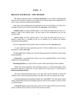
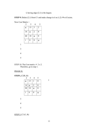
Example 8.1[4-queens] Let us see how a FIFO branch-and-bound algorithm would search
the state space tree (figure 7.2) for the 4-queens problem.
Initially, there is only one live node, node1. This represents the case in which no
queen has been placed on the chessboard. This node becomes the E-node.
It is expanded and its children, nodes2, 18, 34 and 50 are generated.
These nodes represent a chessboard with queen1 in row 1and columns 1, 2, 3, and 4
respectively.
The only live nodes 2, 18, 34, and 50.If the nodes are generated in this order, then the
next E-node are node 2.
2

3. It is expanded and the nodes 3, 8, and 13 are generated. Node 3 is immediately killed
using the bounding function. Nodes 8 and 13 are added to the queue of live nodes.
Node 18 becomes the next E-node. Nodes 19, 24, and 29 are generated. Nodes 19 and
24 are killed as a result of the bounding functions. Node 29 is added to the queue of live
nodes.
Now the E-node is node 34.Figure 8.1 shows the portion of the tree of Figure 7.2 that
is generated by a FIFO branch-and-bound search. Nodes that are killed as a result of the
bounding functions are a "B" under them.
Numbers inside the nodes correspond to the numbers in Figure 7.2.Numbers outside
the nodes give the order in which the nodes are generated by FIFO branch-and-bound.
At the time the answer node, node 31, is reached, the only live nodes remaining are
nodes 38 and 54.
Least Cost (LC) Search:
In both LIFO and FIFO branch-and-bound the selection rule for the next E-node
is rather rigid and in a sense blind. The selection rule for the next E-node does not give
any preference to a node that has a very good chance of getting the search to an answer
node quickly.
Thus, in Example 8.1, when node 30 is generated, it should have become obvious to
the search algorithm that this node will lead to answer node in one move. However, the
rigid FIFO rule first requires the expansion of all live nodes generated before node 30
was expanded.
3

4. The search for an answer node can often be speeded by using an "intelligent" ranking
function (.) for live nodes. The next E-node is selected on the basis of this ranking
function.
If in the 4-queens example we use a ranking function that assigns node 30 a better
rank than all other live nodes, then node 30 will become E-node, following node 29.The
remaining live nodes will never become E-nodes as the expansion of node 30 results in
the generation of an answer node (node 31).
The ideal way to assign ranks would be on the basis of the additional computational
effort (or cost) needed to reach an answer node from the live node. For any node x, this
cost could be
(1) The number of nodes on the sub-tree x that need to be generated before any
answer node is generated or, more simply,
(2) The number of levels the nearest answer node (in the sub-tree x) is from x
Using cost measure (2), the cost of the root of the tree of Figure 8.1 is 4 (node 31 is
four levels from node 1).The costs of nodes 18 and 34,29 and 35,and 30 and 38 are
respectively 3, 2, and 1.The costs of all remaining nodes on levels 2, 3, and 4 are
respectively greater than 3, 2, and 1.
Using these costs as a basis to select the next E-node, the E-nodes are nodes 1, 18, 29,
and 30 (in that order).The only other nodes to get generated are nodes 2, 34, 50, 19, 24,
32, and 31.
The difficulty of using the ideal cost function is that computing the cost of a node
usually involves a search of the sub-tree x for an answer node. Hence, by the time the
cost of a node is determined, that sub-tree has been searched and there is no need to
explore x again. For this reason, search algorithms usually rank nodes only based on an
estimate (.) of their cost.
Let (x) be an estimate of the additional effort needed to reach an answer node from x.
node x is assigned a rank using a function (.) such that (x) =f (h(x)) + (x), where h(x)
is the cost of reaching x from the root and f(.) is any non-decreasing function.
A search strategy that uses a cost function (x) =f (h(x)) + (x), to select the next e-
node would always choose for its next e-node a live node with least (.).Hence, such a
strategy is called an LC-search (least cost search).
Cost function c (.) is defined as, if x is an answer node, then c(x) is the cost (level,
computational difficulty, etc.) of reaching x from the root of the state space tree. If x is
not an answer node, then c(x) =infinity, providing the sub-tree x contains no answer
node; otherwise c(x) is equals the cost of a minimum cost answer node in the sub-tree x.
4

5. It should be easy to see that (.) with f (h(x)) =h(x) is an approximation to c (.). From
now on (x) is referred to as the cost of x.
Bounding:
A branch -and-bound searches the state space tree using any search mechanism in
which all the children of the E-node are generated before another node becomes the E-
node.
We assume that each answer node x has a cost c(x) associated with it and that a
minimum-cost answer node is to be found. Three common search strategies are FIFO,
LIFO, and LC.
A cost function (.) such that (x) <=c(x) is used to provide lower bounds on
solutions obtainable from any node x. If upper is an upper bound on the cost of a
minimum-cost solution, then all live nodes x with (x)>upper may be killed as all
answer nodes reachable from x have cost c(x)>= (x)>upper. The starting value for upper
can be set to infinity.
Clearly, so long as the initial value for upper is no less than the cost of a minimum-
cost answer node, the above rule to kill live nodes will not result in the killing of a live
node that can reach a minimum-cost answer node .Each time a new answer is found ,the
value of upper can be updated.
As an example optimization problem, consider the problem of job scheduling with
deadlines. We generalize this problem to allow jobs with different processing times. We
are given n jobs and one processor. Each job i has associated with it a three tuple
( ).job i requires units of processing time .if its processing is not completed by
the deadline , and then a penalty is incurred.
The objective is to select a subset j of the n jobs such that all jobs in j can be
completed by their deadlines. Hence, a penalty can be incurred only on those jobs not in
j. The subset j should be such that the penalty incurred is minimum among all possible
subsets j. such a j is optimal.
Consider the following instances: n=4,( , , )=(5,1,1),( , , )=(10,3,2),(
, , )=(6,2,1),and( , , )=(3,1,1).The solution space for this instances consists
of all possible subsets of the job index set{1,2,3,4}. The solution space can be organized
into a tree by means of either of the two formulations used for the sum of subsets
problem.
5

6. Figure 8.7
Figure 8.6 corresponds to the variable tuple size formulations while figure 8.7
corresponds to the fixed tuple size formulation. In both figures square nodes represent
infeasible subsets. In figure 8.6 all non-square nodes are answer nodes. Node 9 represents
an optimal solution and is the only minimum-cost answer node .For this node j= {2,3}
and the penalty (cost) is 8. In figure 8.7 only non-square leaf nodes are answer nodes.
Node 25 represents the optimal solution and is also a minimum-cost answer node. This
node corresponds to j={2,3} and a penalty of 8. The costs of the answer nodes of figure
8.7 are given below the nodes.
6

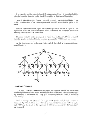
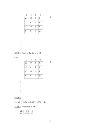
7. TRAVELLING SALESMAN PROBLEM
INTRODUCTION:
It is algorithmic procedures similar to backtracking in which a new branch is
chosen and is there (bound there) until new branch is choosing for advancing.
This technique is implemented in the traveling salesman problem [TSP] which are
asymmetric (Cij <>Cij) where this technique is an effective procedure.
STEPS INVOLVED IN THIS PROCEDURE ARE AS FOLLOWS:
STEP 0: Generate cost matrix C [for the given graph g]
STEP 1: [ROW REDUCTION]
For all rows do step 2
STEP: Find least cost in a row and negate it with rest of the
elements.
STEP 3: [COLUMN REDUCTION]
Use cost matrix- Row reduced one for all columns do STEP 4.
STEP 4: Find least cost in a column and negate it with rest of the elements.
STEP 5: Preserve cost matrix C [which row reduced first and then column reduced]
for the i th
time.
STEP 6: Enlist all edges (i, j) having cost = 0.
STEP 7: Calculate effective cost of the edges. ∑ (i, j)=least cost in the i th
row
excluding (i, j) + least cost in the j th
column excluding (i, j).
STEP 8: Compare all effective cost and pick up the largest l. If two or more have
same cost then arbitrarily choose any one among them.
STEP 9: Delete (i, j) means delete ith
row and jth
column change (j, i) value to
infinity. (Used to avoid infinite loop formation) If (i,j) not present, leave it.
STEP 10: Repeat step 1 to step 9 until the resultant cost matrix having order of 2*2
and reduce it. (Both R.R and C.C)
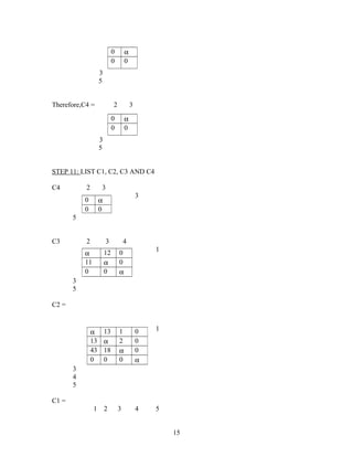
STEP 11: Use preserved cost matrix Cn, Cn-1… C1
7

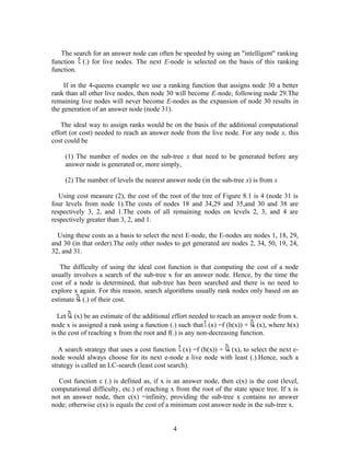
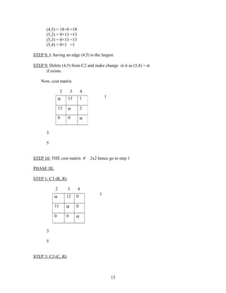
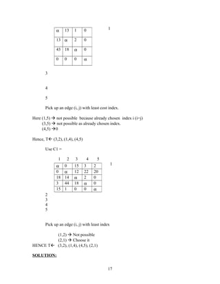
8. Choose an edge [i, j] having value =0, at the first time for a preserved
matrix and leave that matrix.
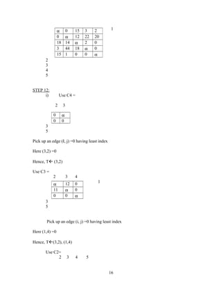
STEP 12: Use result obtained in Step 11 to generate a complete tour.
EXAMPLE: Given graph G
22 5
27 25
9 19
25
8
1
50
10 31 17 15
6 40
30
7
6
24
MATRIX:
1 2 3 4 5
1
2
3
4
5
8
α 25 40 31 27
5 α 17 30 25
19 15 α 6 1
9 50 24 α 6
22 8 7 10 α
1
5 2
4 3

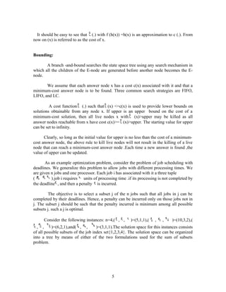
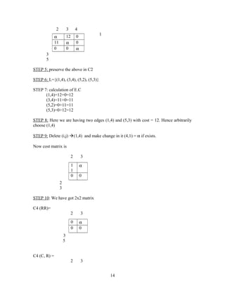
9. PHASE I
STEP 1: Row Reduction C
C1 [ROW REDUCTION:
1 2 3 4 5
1
2
3
4
5
STEP 3: C1 [Column Reduction]
1 2 3 4 5
1
9
α 0 15 6 2
0 α 12 25 20
18 14 α 5 0
3 44 18 α 0
15 1 0 3 α
α 0 15 3 2
0 α 12 2
5
20
18 14 α 2 0
3 44 18 α 0
15 1 0 3 α

10. 2
3
4
5
STEP 5:
Preserve the above in C1,
1 2 3 4 5
1
2
3
4
5
STEP 6:
L= { }(5,4)(5,3),(4,5),(3,5),(2,1),(1,2),
STEP 7:
Calculation of effective cost [E.C]
(1,2) = 2+1 =3
(2,1) = 12+3 = 15
(3,5) = 2+0 =2
(4,5) = 3+0 = 3
(5,3) = 0+12 = 12
(5,4) = 0+2 = 2
STEP 8:
10
α 0 15 3 2
0 α 12 22 20
18 14 α 2 0
3 44 18 α 0
15 1 0 3 α

11. L having edge (2,1) is the largest.
STEP 9: Delete (2,1) from C1 and make change in it as (1,2)  α if exists.
Now Cost Matrix =
2 3 4 5
1
3
4
5
STEP 10: The Cost matrix ≠ 2 x 2.
Therefore, go to step 1.
PHASE II:
STEP1: C2(R, R)
2 3 4 5
1
3
4
5
STEP 3: C2 (C, R)
11
α 15 3 2
14 α 2 0
44 18 α 0
1 0 0 α
α 13 1 0
14 α 2 0
44 18 α 0
1 0 0 α

12. 2 3 4 5
1
3
4
5
STEP 5: Preserve the above in C2
C2 =
2 3 4 5
1
3
4
5
STEP 6:
L= {(1,5), (3,5), (4,5), (5,2), (5,3), (5,4)}
STEP 7: calculation of E.C.
(1,5) = 1+0 =1
(3,5) = 2+0 =2
12
α 13 1 0
13 α 2 0
43 18 α 0
0 0 0 α
α 13 1 0
13 α 2 0
43 18 α 0
0 0 0 α

13. (4,5) = 18+0 =18
(5,2) = 0+13 =13
(5,3) = 0+13 =13
(5,4) = 0+1 =1
STEP 8: L having an edge (4,5) is the largest.
STEP 9: Delete (4,5) from C2 and make change in it as (5,4) = α
if exists.
Now, cost matrix
2 3 4
1
3
5
STEP 10: THE cost matrix ≠ 2x2 hence go to step 1
PHASE III:
STEP 1: C3 (R, R)
2 3 4
1
3
5
STEP 3: C3 (C, R)
13
α 13 1
13 α 2
0 0 α
α 12 0
11 α 0
0 0 α

14. 2 3 4
1
3
5
STEP 5: preserve the above in C2
STEP 6: L={(1,4), (3,4), (5,2), (5,3)}
STEP 7: calculation of E.C
(1,4)=12+0=12
(3,4)=11+0=11
(5,2)=0+11=11
(5,3)=0+12=12
STEP 8: Here we are having two edges (1,4) and (5,3) with cost = 12. Hence arbitrarily
choose (1,4)
STEP 9: Delete (i,j) (1,4) and make change in it (4,1) = α if exists.
Now cost matrix is
2 3
2
3
STEP 10: We have got 2x2 matrix
C4 (RR)=
2 3
3
5
C4 (C, R) =
2 3
14
α 12 0
11 α 0
0 0 α
1
1
α
0 0
0 α
0 0

15. 3
5
Therefore,C4 = 2 3
3
5
STEP 11: LIST C1, C2, C3 AND C4
C4 2 3
3
5
C3 2 3 4
1
3
5
C2 =
1
3
4
5
C1 =
1 2 3 4 5
15
0 α
0 0
0 α
0 0
0 α
0 0
α 12 0
11 α 0
0 0 α
α 13 1 0
13 α 2 0
43 18 α 0
0 0 0 α

16. 1
2
3
4
5
STEP 12:
i) Use C4 =
2 3
3
5
Pick up an edge (I, j) =0 having least index
Here (3,2) =0
Hence, T (3,2)
Use C3 =
2 3 4
1
3
5
Pick up an edge (i, j) =0 having least index
Here (1,4) =0
Hence, T(3,2), (1,4)
Use C2=
2 3 4 5
16
α 0 15 3 2
0 α 12 22 20
18 14 α 2 0
3 44 18 α 0
15 1 0 0 α
0 α
0 0
α 12 0
11 α 0
0 0 α

17. 1
3
4
5
Pick up an edge (i, j) with least cost index.
Here (1,5)  not possible because already chosen index i (i=j)
(3,5)  not possible as already chosen index.
(4,5) 0
Hence, T (3,2), (1,4), (4,5)
Use C1 =
1 2 3 4 5
1
2
3
4
5
Pick up an edge (i, j) with least index
(1,2)  Not possible
(2,1)  Choose it
HENCE T (3,2), (1,4), (4,5), (2,1)
SOLUTION:
17
α 13 1 0
13 α 2 0
43 18 α 0
0 0 0 α
α 0 15 3 2
0 α 12 22 20
18 14 α 2 0
3 44 18 α 0
15 1 0 0 α

18. From the above list
3—2—1—4—5
This result now, we have to return to the same city where we started (Here 3).
Final result:
3—2—1—4—5—3
Cost is 15+15+31+6+7=64
18