This paper explores kakuro as a constraint satisfaction problem, presenting a formal representation of its constraints and a solution approach using concepts like i-consistency and backtracking search. The authors compare the efficiency of their heuristic methods against naive brute-force approaches, demonstrating improved runtime performance through preprocessing and variable selection heuristics. The study concludes that the proposed algorithm significantly outperforms traditional methods, showcasing the effectiveness of constraint formulation and solving techniques.

1. Kakuro: Solving the Constraint Satisfaction
Problem∗
Prateek Jain, Rohit Malhotra, Varad Meru
University of California, Irvine
{prateekj,rohitm,vmeru}@uci.edu
Abstract
In this paper we describe Kakuro as a constraint problem. We’ve cre-
ated a formal representation expressing constraints of the problem and
developed an approach to solve the problem using constraint solving con-
cepts such as i-consistency, forward checking, constraint propagation and
most restrained value heuristics. We also do a comparative analysis of
naive brute force and our heuristics based approach.
1 Introduction
Kakuro is a mathematical logic puzzle often seen as the mathematical trans-
lation of crosswords. It is one of the many logical puzzles popularized by the
Japanese company Nikoli[2].It is one of the oldest grid logic puzzles, its existence
can be traced back to the April/May 1950 issue of Official Crossword Puzzles
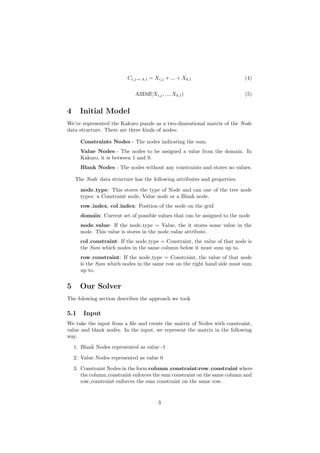
by Dell Publishing Company, and was called as Cross-Sums[1]. Figure 1 shows
a small scale example taken from [3] and its solution.
The puzzle is described by the following rules:
∗This work was done as a part of the project for the course CS 271: Introduction to
Artificial Intelligence, taught in Fall 2014 by Prof. Kalev Kask.
Figure 1: Example Problem and Solution
1

2. 1. The puzzle consists of a rectilinear grid of black and white cells. Black
cells may contain hints (integer numbers). The number below the diag-
onal divider is the sum constraint for cells below, the number above the
diagonal divider is the sum constraint for cells to the right.
2. The task is to enter numbers from 1 to 9 into the white cells satisfying
the following constraints:
(a) The sum of a continuous block of white cells in horizontal (or vertical)
direction must be equal to the constraint given in the black cell to
the left (or above).
(b) All numbers in a continuous block of white cells must be pairwise
different.
The grid size of the puzzle can vary, ranging from the smallest interesting
puzzle of size 5-by-5, to giant puzzles of size 30-by-30. A typical size for human
is around 9-15 cells square[4]. A valid Kakuro puzzle has solutions, a well posed
problem admits a single solution. A finite set of deduction rules are sufficient in
deducing the solution to the posed question without using search. An interesting
feature of logical puzzles is that the solution should be deduced with a finite set
of deduction rules, without using search. A characterisation of the difficulty of
a puzzle instance is the rule set required to solve it.
2 Related Work
Kakuro has become widely popular in the wake of the craze behind puzzle
games like Sudoku[3]. While most of the number puzzles are about constraint
satisfaction, their are significantly different in their problem structure. Sudoku
is mainly concerned with the propagation of the alldifferent constraint and the
interaction of multiple such constraints[5, 6], while Kakuro is a combination of
an alldifferent constraint with the sum constraint over the same variables. The
alldifferent-sum constraint is not found in the global constraint catalog [2].
3 Problem Formulation
Kakuro is essentially a constraint satisfaction problem that can be formally
represented in terms of variables with constraints between them that .must be
satisfied in
V ariables = Xi,j (1)
1 refers to value inside i, jth
cell.
Constraints = Ci,j→ k,l (2)
2 refers to a constraint applicable on variables Xi,j to Xk,l
Constraints in Kakuro are integers. All the variables that are bound by a
common constraint must be different from each other and add up to the sum
specified by that constraint.
Xi,j ∈ {1, 2, 3, 4, 5, 6, 7, 8, 9} (3)
2

3. Ci,j→ k,l = Xi,j + ... + Xk,l (4)
AllDiff(Xi,j, ..., Xk,l) (5)
4 Initial Model
We’ve represented the Kakuro puzzle as a two-dimentional matrix of the Node
data structure. There are three kinds of nodes:
Constraints Nodes - The nodes indicating the sum.
Value Nodes - The nodes to be assigned a value from the domain. In
Kakuro, it is between 1 and 9.
Blank Nodes - The nodes without any constraints and stores no values.
The Node data structure has the following attributes and properties:
node type: This stores the type of Node and can one of the tree node
types: a Constraint node, Value node or a Blank node.
row index, col index: Position of the node on the grid
domain: Current set of possible values that can be assigned to the node
node value: If the node type = Value, the it stores some value in the
node. This value is stores in the node value attribute.
col constraint: If the node type = Constraint, the value of that node is
the Sum which nodes in the same column below it must sum up to.
row constraint: If the node type = Constraint, the value of that node
is the Sum which nodes in the same row on the right hand side must sum
up to.
5 Our Solver
The folowing section describes the approach we took
5.1 Input
We take the input from a file and create the matrix of Nodes with constraint,
value and blank nodes. In the input, we represent the matrix in the following
way.
1. Blank Nodes represented as value -1
2. Value Nodes represented as value 0
3. Constraint Nodes in the form column constraint:row constraint where
the column constraint enforces the sum constraint on the same column and
row constraint enforces the sum constraint on the same row.
3

4. Figure 2: A sample row-column pair.
5.2 Local i-consistency
After taking the input, as specified in 5.1, we take each constraint node one
by one, and make all the nodes constrained by that Sum constraint consistent
with each other. We present the following mathematical model for establishing
general i-consistency between nodes.
Lets take a row with row constraints in the Kakuro Puzzle. The value nodes
between two constraint nodes are constrained by the Sum of the row constraint
of the left constraint node.
Let the value of the Total Sum for the row constraint be S.
Let the number of value nodes which have no value assigned be i
Then chosing any 1 of the value nodes in the row, the sum of the remaining
i − 1 nodes can be a minimum of 1+2+...(i-1)
S =
i−1
n=1
n = i(i − 1)/2 (6)
Hence the value of the chosen value node cannot be greater than
MaxVal = Sum - (i(i-1)/2)
Hence we eliminate the values greater than MaxVal from that domain of all
the i nodes. Similarly, chosing any 1 of the value nodes in the row, the sum of
the remaining nodes can be a maximum of 9+8+..(10-i)
S =
i−1
n=1
(10 − n) = (20 − i)(i − 1)/2 (7)
Hence the value of the chosen value node cannot be less than
MinV al = Sum − ((20 − i)(i − 1)/2). Therefore, we eliminate all domain
values from all the value nodes which are less than MinVal.
4

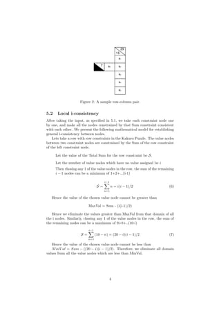
5. Figure 3: Constraint Graph of the sample row-column pair from 2.
5.3 Creating the constraint graph
After we have reduced the domain of the value nodes through local i-consistency,
we create the constraint graph for the problem. Instead of following the ap-
proach of traversing through the graph for value nodes and creating the adja-
cency list for each of them, we follow a more efficient approach for creating the
constraint graph. We traverse through the matrix to look for constraint nodes.
When we find a constraint node, we traverse along the row for row constraint
and along column for column constraint. During the traversal, we keep a track
of all value nodes in the path till a new constraint node or a blank node is
reached. We then add each node in the list, to each other’s adjacency list while
avoiding duplicate edges.The elements in the adjacency list are stored in the
form of tuples of (i,j) which correspond to the indices of the Node in the Ma-
trix. For example :- For the part of the Kakuro puzzle shown in Figure 2, the
following is the snapshot of the adjacency list
x1: [x2, x3, x4, x5]
x2: [x1, x3, x4, x5, x6]
x3: [x1, x2, x4,x5]
x4: [x1, x2, x3, x5]
x5: [x1, x2, x3, x4, x5]
5.4 Backtracking Search
We use BackTracking Search to search for the assignment that satisfies all con-
straints. Like a typical, Backtracking algorithm, we have a SELECT-UNASSIGNED-
VARIABLE strategy which picks up the next variable to be selected for assigning
the value from its domain. For the initial approach, we start with the first cell
X0,0, and then we go to the next variable in the same row till the end of the
row. Then we move to next row. This continues till the last variable is assigned
the value.
Once a variable is selected for assignment, we create a copy of its domain
and the domains of all the nodes which are constrained by that variable. We do
this by going through the adjacency list of the assigned node.
5

6. Puzzle X Y C V Min Time (in S) Max Time (in S) Average (in S)
1 3 3 4 4 0.004730225 0.008662939 0.006304693
2 3 3 3 4 0.000432014 0.000535965 0.000467539
3 4 4 5 8 0.003899097 0.007289171 0.005249619
4 7 6 14 24 0.186563015 0.226837158 0.205242252
5 8 8 20 36 10.72893 11.31279707 11.0450578
6 12 10 41 73 18.20192695 25.81185603 20.30568962
Table 1: Brute Force Search. X = Rows, Y = Columns, C = Constraint Nodes,
V = Value Nodes
Once, we assign the value to the node, we then apply Forward Checking
to eliminate the assigned value from the domains of all the adjacent variables
from the constraint graph.
After applying the Forward Checking, we apply Contraint Propogation
to check if any of the constraints including the Sum constraint is violated for any
of the constraint nodes. If a constraint is violated, the domain of the affected
variables is restored to its original value and the next value from the domain
is chosen. If, the constraint is not violated, the algorithm picks up the next
variable to be assigned and calls the BackTrackingSearch recursively. If none
of the values of the domain satisfy the constraint, the BackTracking search
algorithm returns false.
5.5 Improving search through heuristic
Chosing the next variable in the row for assignment is an inefficient way for vari-
able selection. For improving the efficiency of our search algorithm, we employ
the Minimum Remaining Values hueristic. We chose the variable whose
domain is the smallest as the next variable to be assigned. For implementing
this heuristic, we use a priority queue using HeapQ library from python. The
priority in the heap is set to be the size of the domain of the variables.
6 Experimental Results
We test our model on a selection of different configurations of the puzzle.
Puzzle 1 : 3-by-3; Constraint Nodes = 4; Value Nodes = 4.
Puzzle 2 : 3-by-3; Constraint Nodes = 3; Value Nodes = 4.
Puzzle 3 : 4-by-4; Constraint Nodes = 5; Value Nodes = 8.
Puzzle 4 : 7-by-6; Constraint Nodes = 14; Value Nodes = 24.
Puzzle 5 : 8-by-8; Constraint Nodes = 20; Value Nodes = 36.
Puzzle 6 : 12-by-10; Constraint Nodes = 41; Value Nodes = 73.
The problem sizes range from very small (3x3 grid with 36 variables) to quite
large (12 rows, 10 columns and 73 variables). The experiments for all systems
were run on a laptop with 2.4GHz Core i5 processor and 8Gb of memory under
Mac OS X.
6

7. (a) Puzzle 1 (b) Puzzle 2
(c) Puzzle 3 (d) Puzzle 4
(e) Puzzle 5 (f) Puzzle 6
Figure 4: Running Various Experiments. The three bars are for Brute Force,
I-Consistency and I-Consistency with MRV search. All the times given are in
Seconds
7

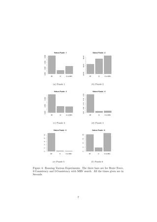
8. Puzzle X Y C V Min Time (in S) Max Time (in S) Average
1 3 3 4 4 0.000769138 0.001533985 0.001207948
2 3 3 3 4 0.000556946 0.00100112 0.000729728
3 4 4 5 8 0.001512051 0.002784014 0.001809359
4 7 6 14 24 0.013028145 0.021849871 0.015318632
5 8 8 20 36 0.251662016 0.316115856 0.273978305
6 12 10 41 73 1.231163979 7.809942961 4.393643355
Table 2: Search with i-consistency check. X = Rows, Y = Columns, C =
Constraint Nodes, V = Value Nodes
Puzzle X Y C V Min Time (in S) Max Time (in S) Average
1 3 3 4 4 0.000720024 0.0075984 0.002657723
2 3 3 3 4 0.000557899 0.00230813 0.000879169
3 4 4 5 8 0.001368999 0.002490997 0.001717162
4 7 6 14 24 0.013787031 0.0273211 0.019261742
5 8 8 20 36 0.146360874 0.189740181 0.1664819
6 12 10 41 73 17.07698488 25.09361315 21.82159901
Table 3: Search with i-consistency check and MRV heuristic. X = Rows, Y =
Columns, C = Constraint Nodes, V = Value Nodes
7 Conclusion
Based on the runtime analysis, our algorithm works way better than brute force
approach. Most gains seen are due to the preprocessing domain reduction step
through i-consistency. We also find further improvements in runtime while using
the Minimum Remaining Values hueristic in 5 out of 6 cases. Our algorithm
provides an efficient way to solve the Kakuro puzzle by formulating the puzzle as
a Constraint Satisfaction problem and applying concepts such as i-consistency,
Forward Checking, Constraint Propagation and Minimum Remaining Values
heuristics. As seen from the results, the approach provides better runtime than
naive brute force and search without hueristics.
References
[1] Shortz, Will, Will Shortz Presents Easy Kakuro: 100 Addictive Logic Puz-
zles, 2006.
[2] Nikoli web site, http://www.nikoli.co.jp/en/puzzles/index.html, ac-
cessed on 2014-12-14.
[3] Wikipedia page on Kakuro, http://en.wikipedia.org/wiki/Kakuro, ac-
cessed on 2014-12-14.
[4] Huckvale, Mark. Kakuro Puzzles webpage,
http://www.phon.ucl.ac.uk/home/mark/kakuro/, accessed on 2014-
12-14.
8

9. [5] Simonis, Helmut. Sudoku as a constraint problem, CP Workshop on modeling
and reformulating Constraint Satisfaction Problems. Vol. 12, 2005.
[6] Lynce, Inˆes, and Ouaknine, Jo¨el. Sudoku as a SAT Problem ISAIM. 2006.
[7] Beldiceanu, Nicolas, Carlsson, Mats, and Rampon, Jean-Xavier. Global con-
straint catalog, (revision a). (2012).
9