Download as PDF, PPTX
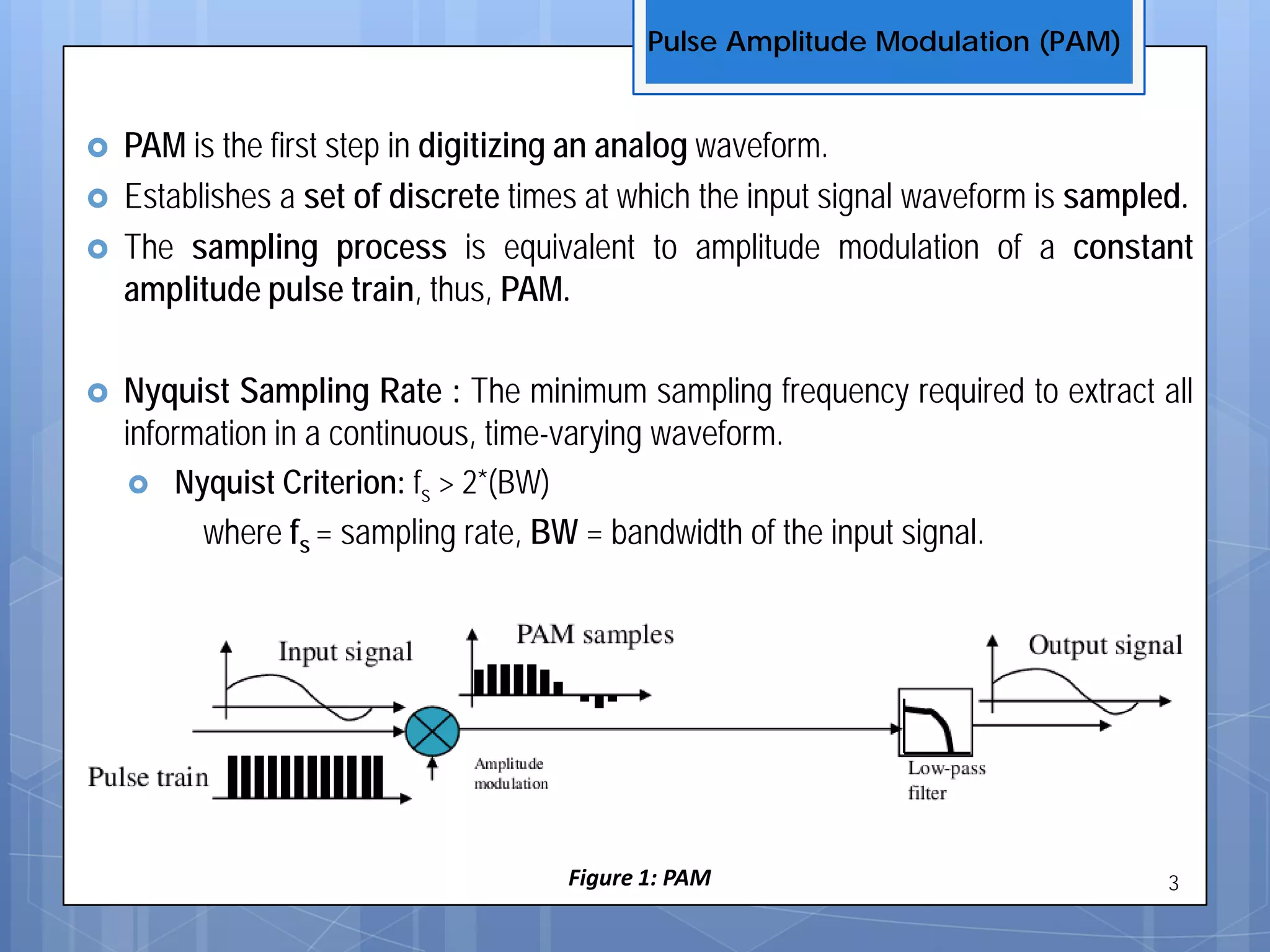


1) Pulse amplitude modulation (PAM) is used to digitize analog voice signals by sampling the amplitude of the voice waves at discrete time intervals. 2) For faithful reproduction of the original analog signal, the sampling rate must be at least twice the highest frequency component of the voice signal, as per the Nyquist criterion. 3) If the sampling rate is lower than the Nyquist rate, aliasing or foldover distortion will occur, distorting the reconstructed signal.
Introduction to the presentation on telecommunications by the instructor Md Hasib Noor in the context of the Faculty of Engineering.
Voice is analog, characterized by amplitude, frequency, and phase. Digitization improves quality, capacity and distance.
PAM samples analog waveforms at discrete times. Introduces Nyquist Sampling Rate and Criterion related to bandwidth.
Differentiation between Nyquist frequency and Nyquist rate, emphasizing the importance of sampling rates in signal processing.
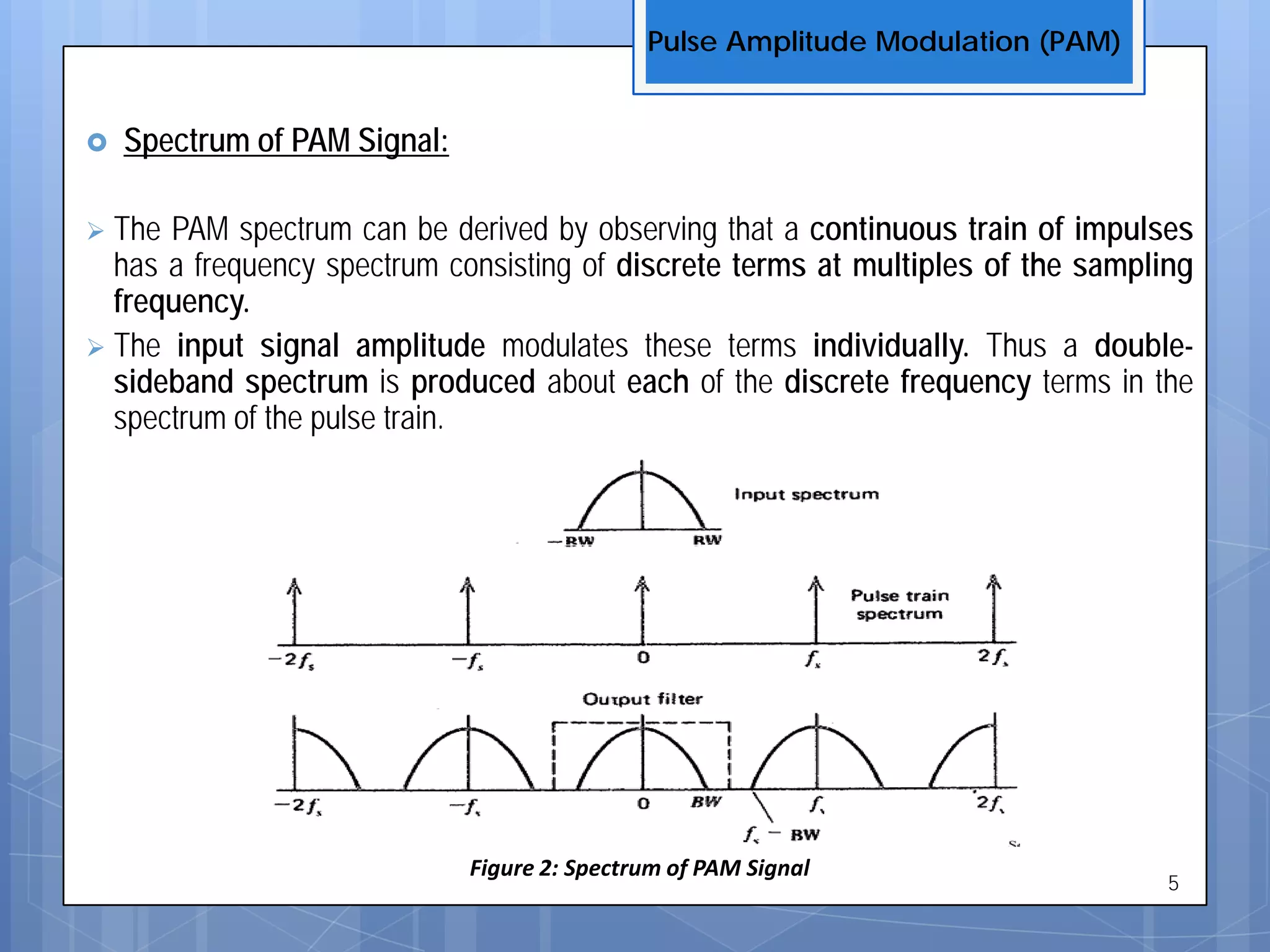
The frequency spectrum of PAM signals, derived from a continuous pulse train and its effects on signal representation.
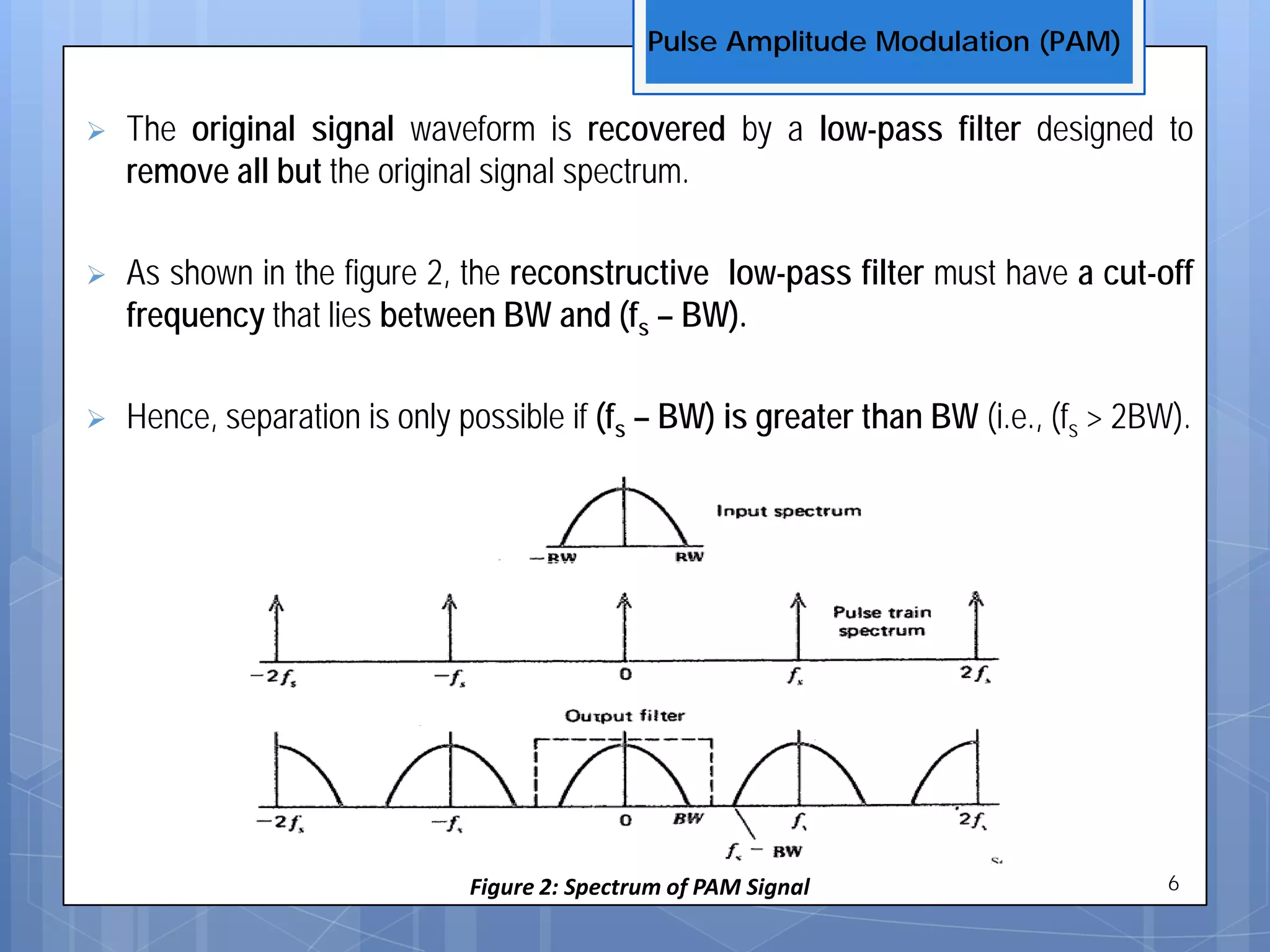
Discusses the necessity of a low-pass filter to recover the original signal from PAM while maintaining specific cutoff frequencies.
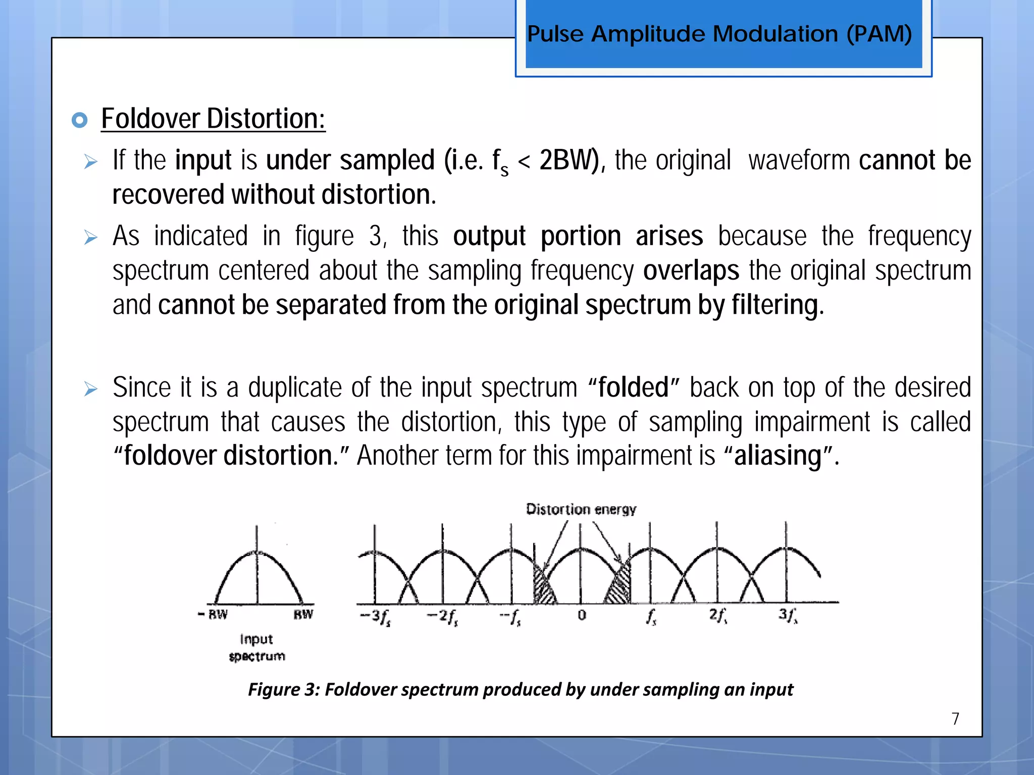
Describes foldover distortion or aliasing resulting from under sampling where original waveforms cannot be accurately recovered.
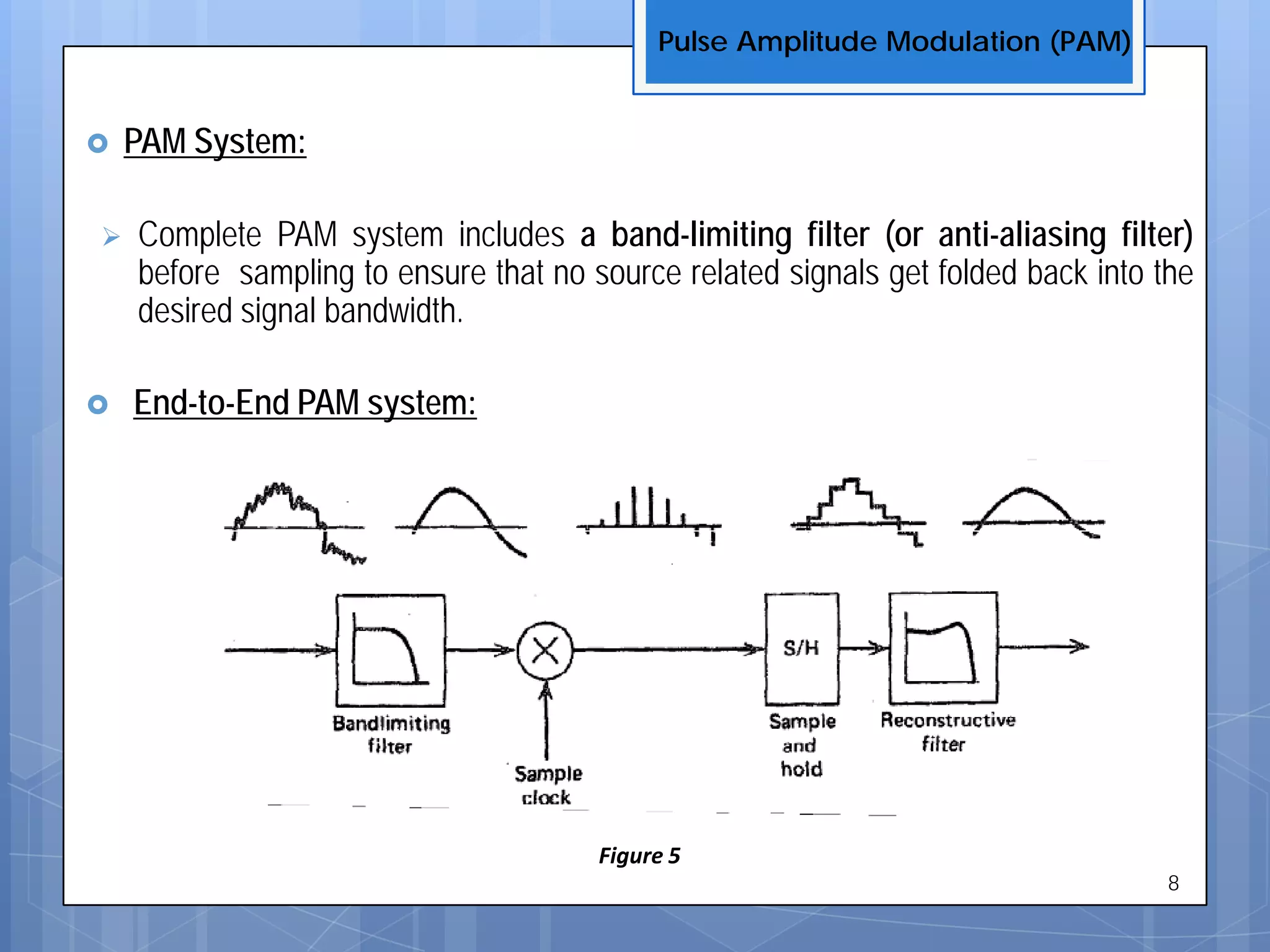
Overview of PAM systems, including the need for band-limiting filters to avoid aliasing during sampling.
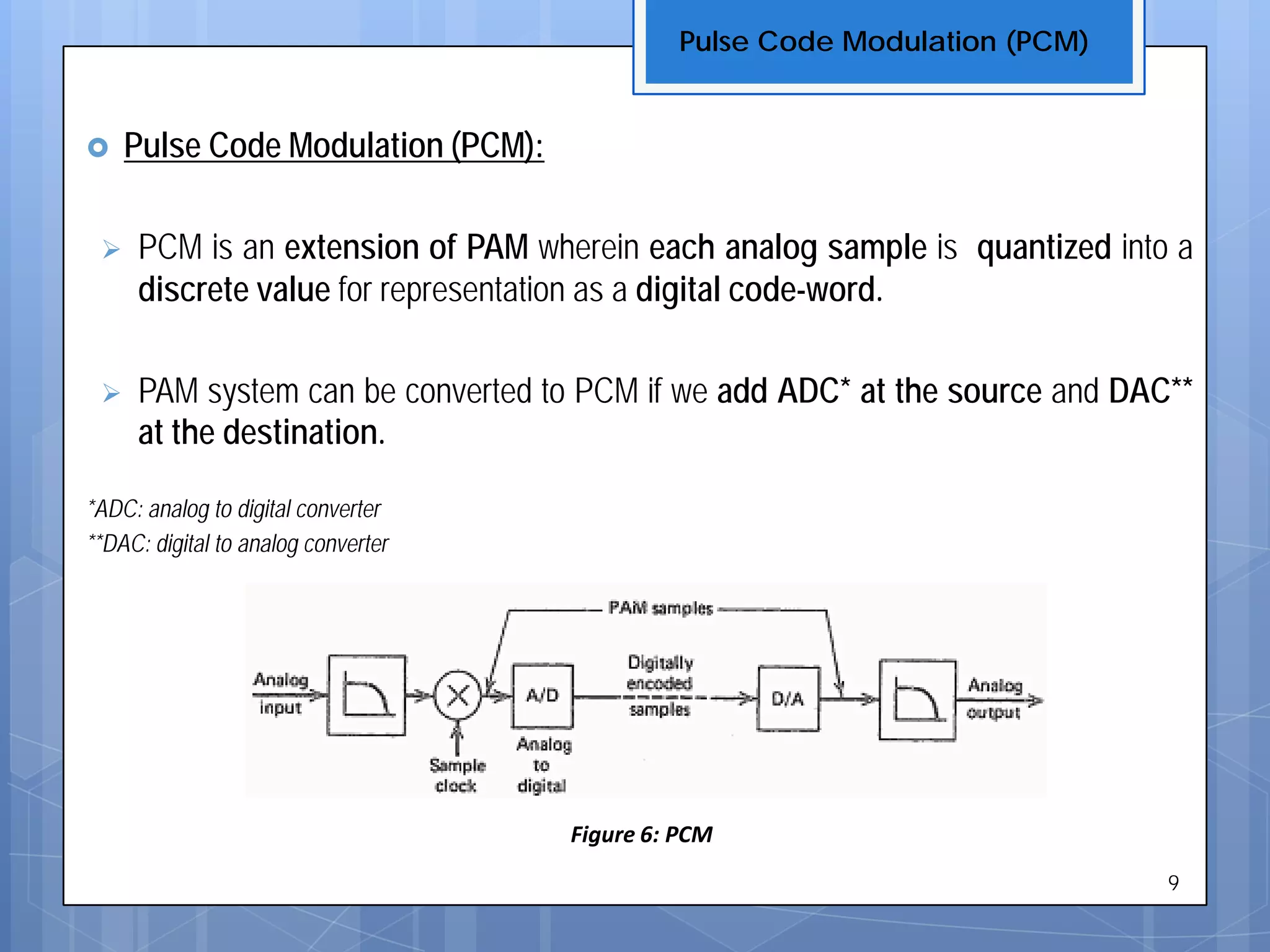
PAM's extension to PCM, which quantizes each analog sample into discrete values represented as digital code-words.
Discusses PAM's vulnerabilities over long distances and introduces finite bit representation of PAM sample amplitudes.
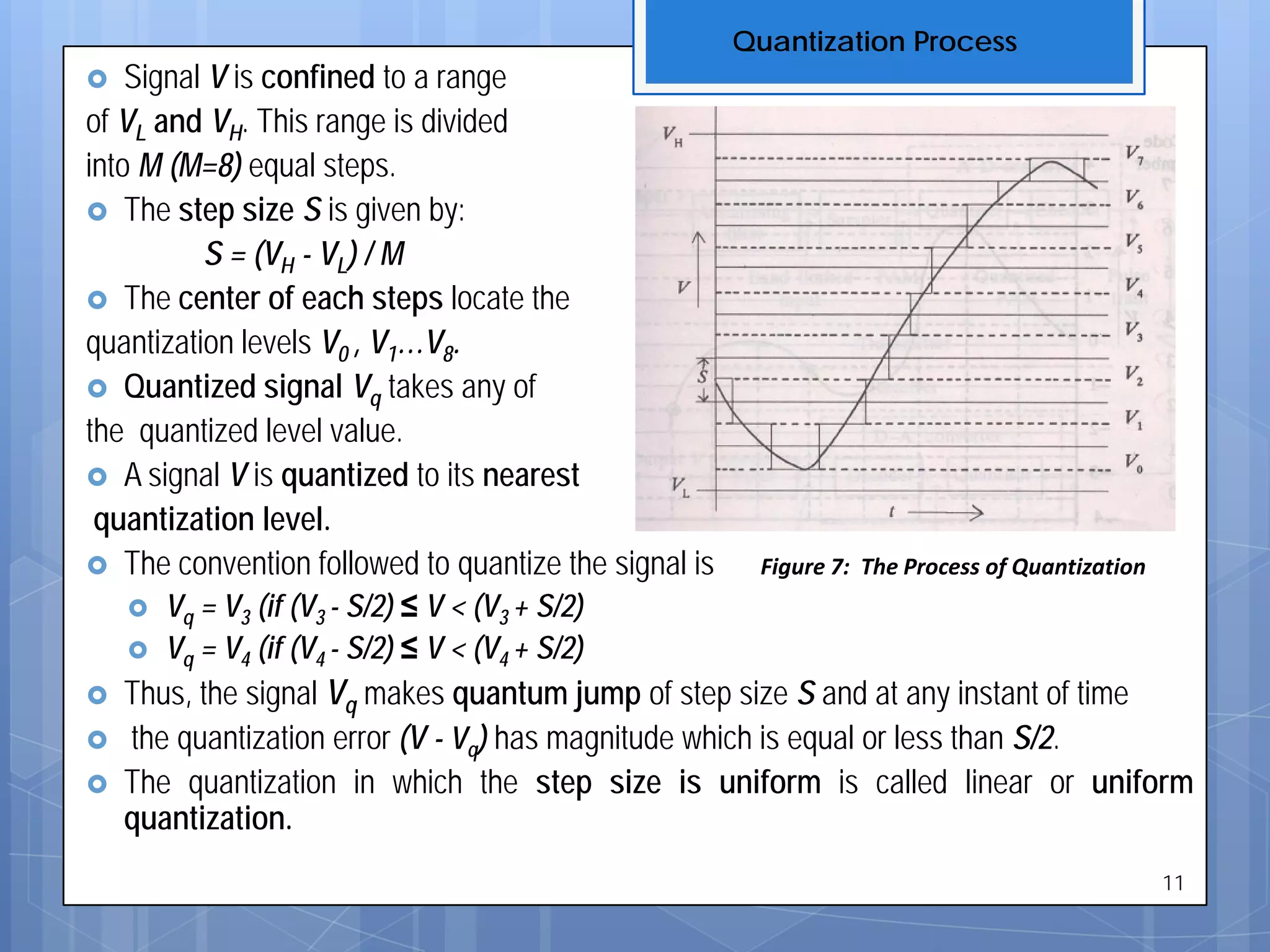
Explains how signals are quantized into discrete levels, representing quantization errors and the concept of uniform quantization.
Examines quantization noise and the use of repeaters to maintain signal integrity amid noise and quantization levels.
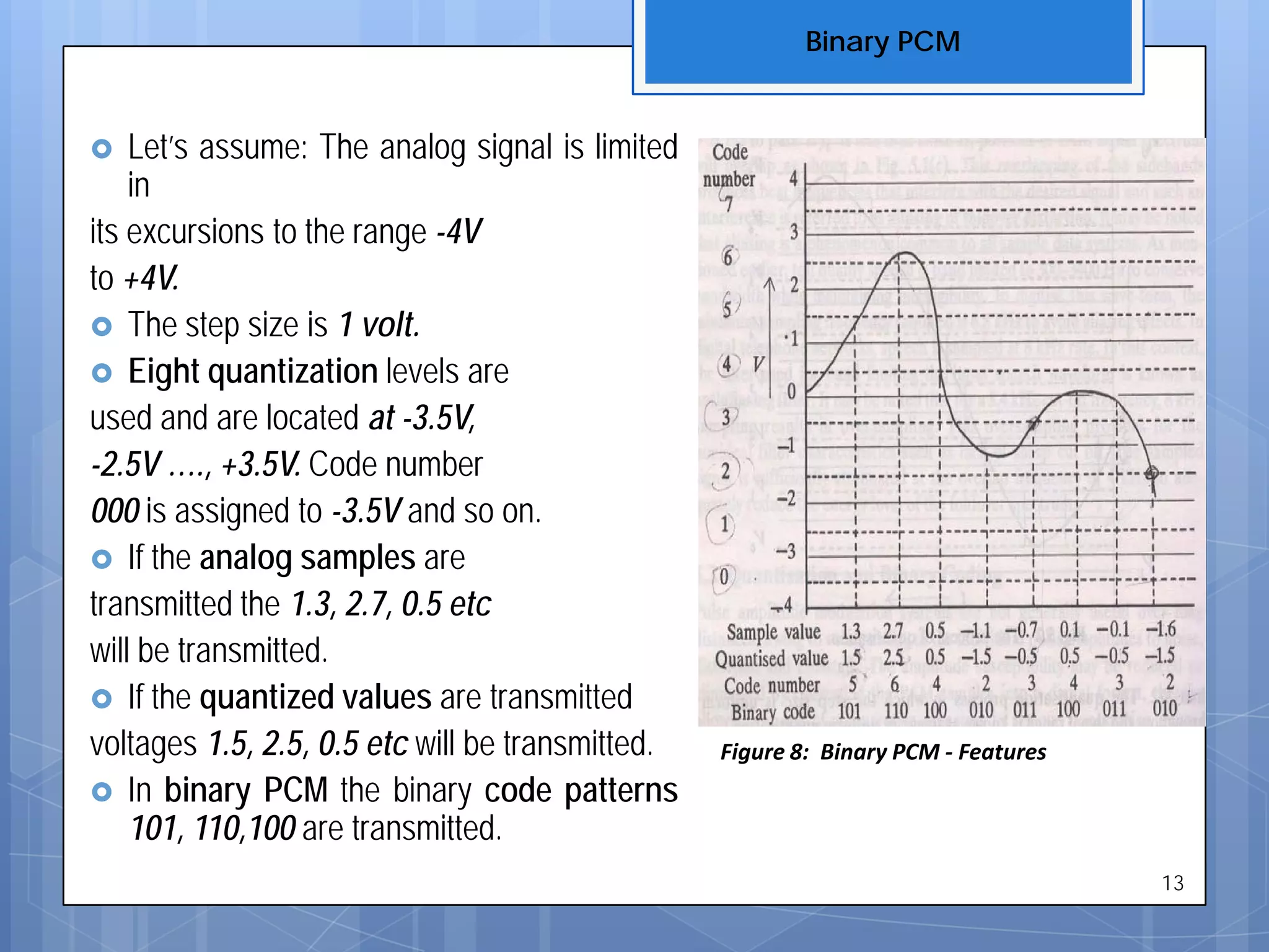
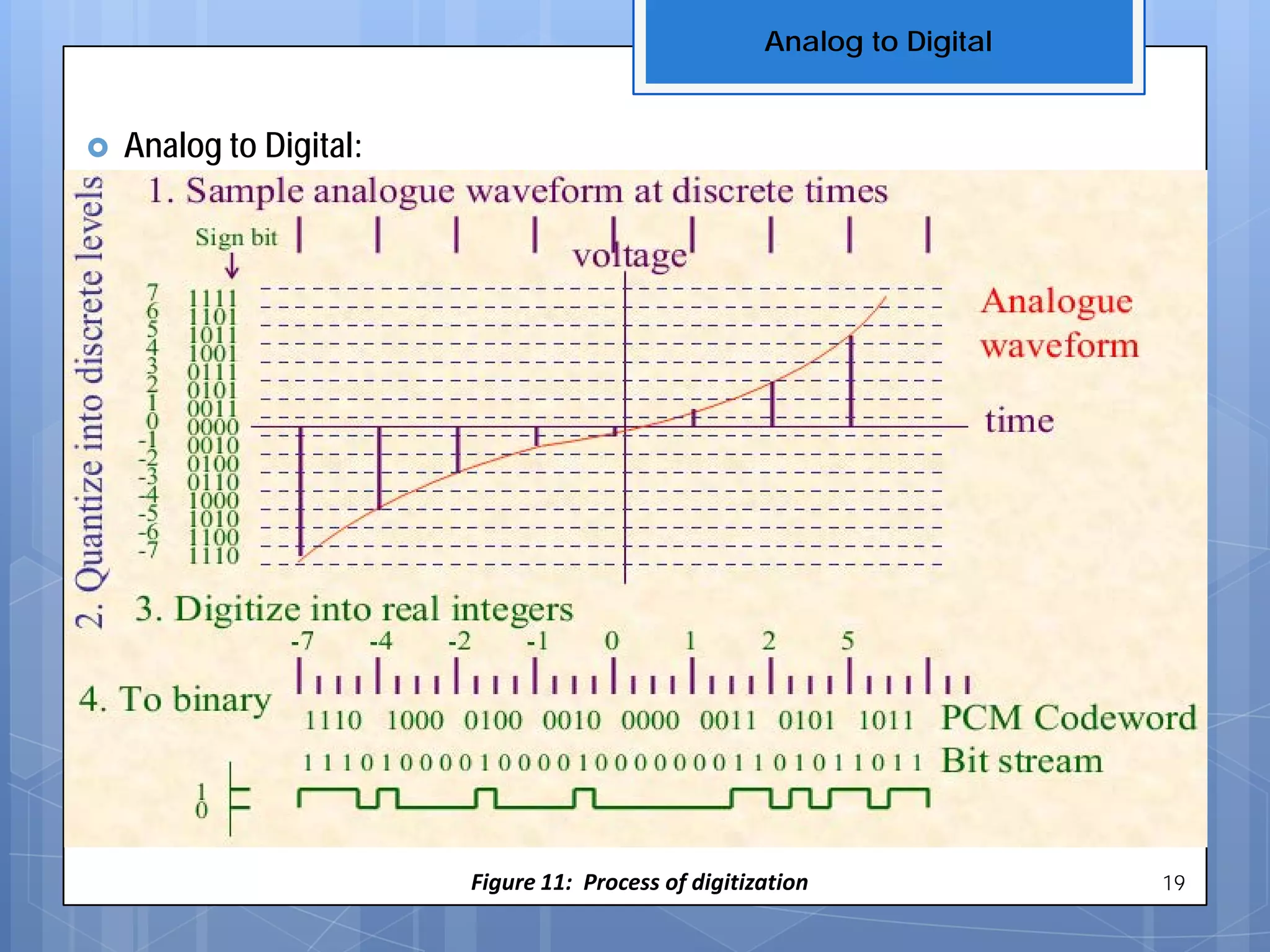
Illustrates the process of transmitting analog signals as quantized and binary PCM code patterns.
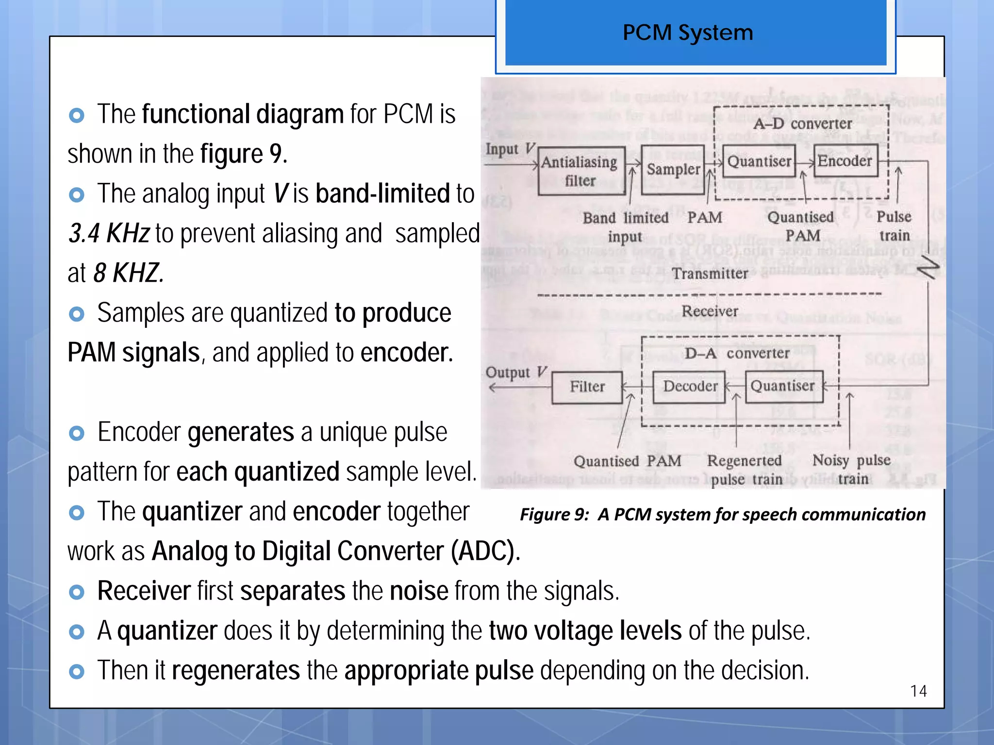
Describes the functional components of a PCM system including ADC and signal recovery processes at the receiver.
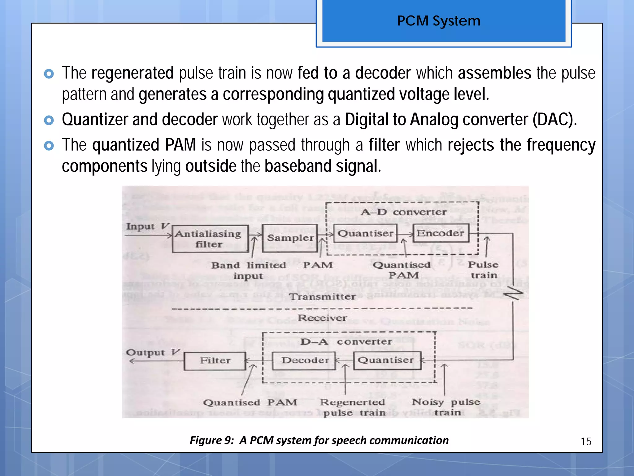
Continues the explanation of the PCM process focusing on the role of decoders and filters in reconstructing signals.
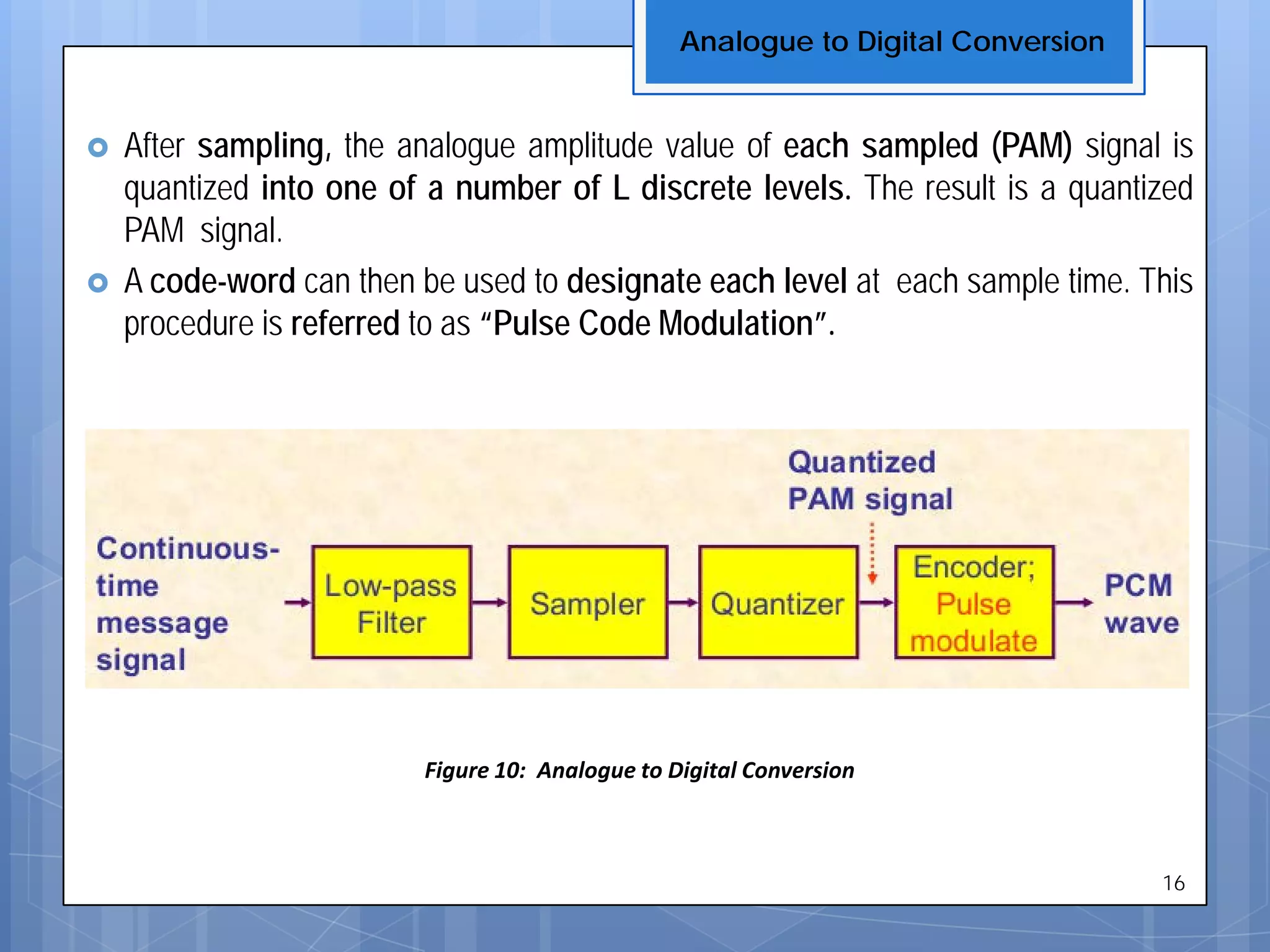
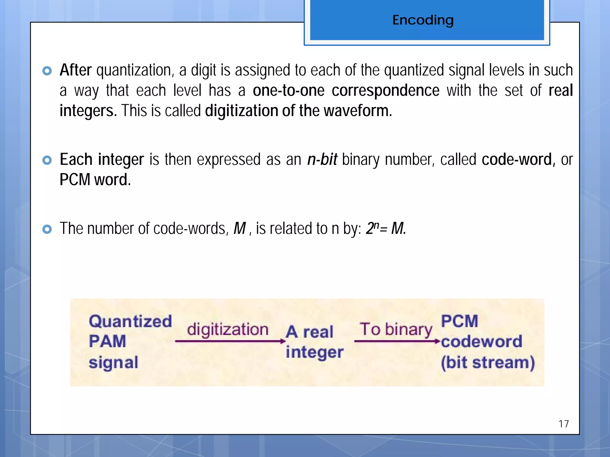
Describes the entire process of converting analog signals to digital code-words through sampling and quantization.
Details the mapping of quantized amplitudes into corresponding PCM code-words as part of the digitization process.
Introduces the concept of codebooks containing codewords for quantized signal levels in PCM.
Discusses quantization noise as an approximation error in signal representation and its characteristics.
Examines the distribution of quantization noise and the statistical characteristics affecting PCM system performance.
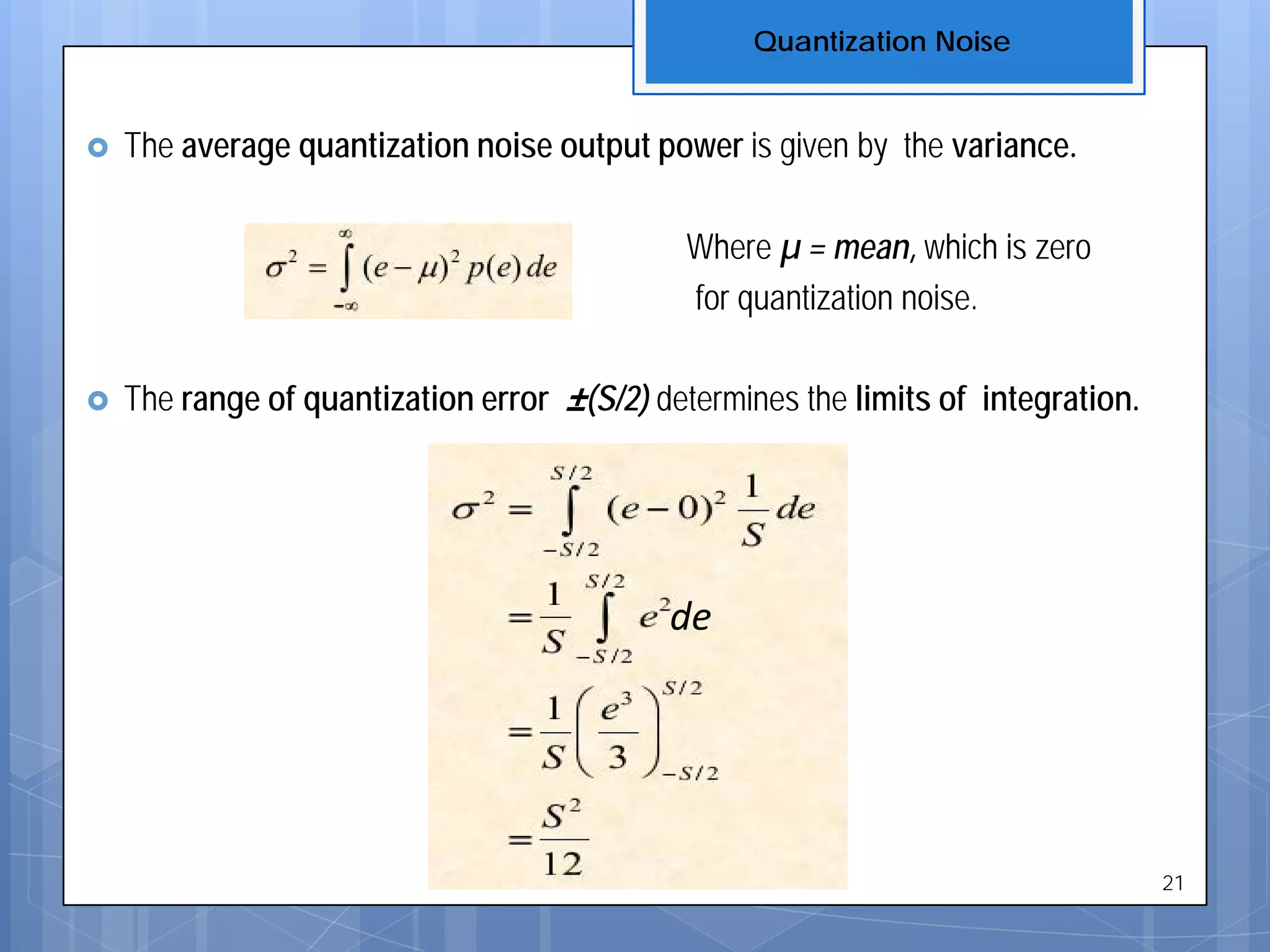
Provides a mathematical basis for quantization noise measurements and variance in PCM signals.
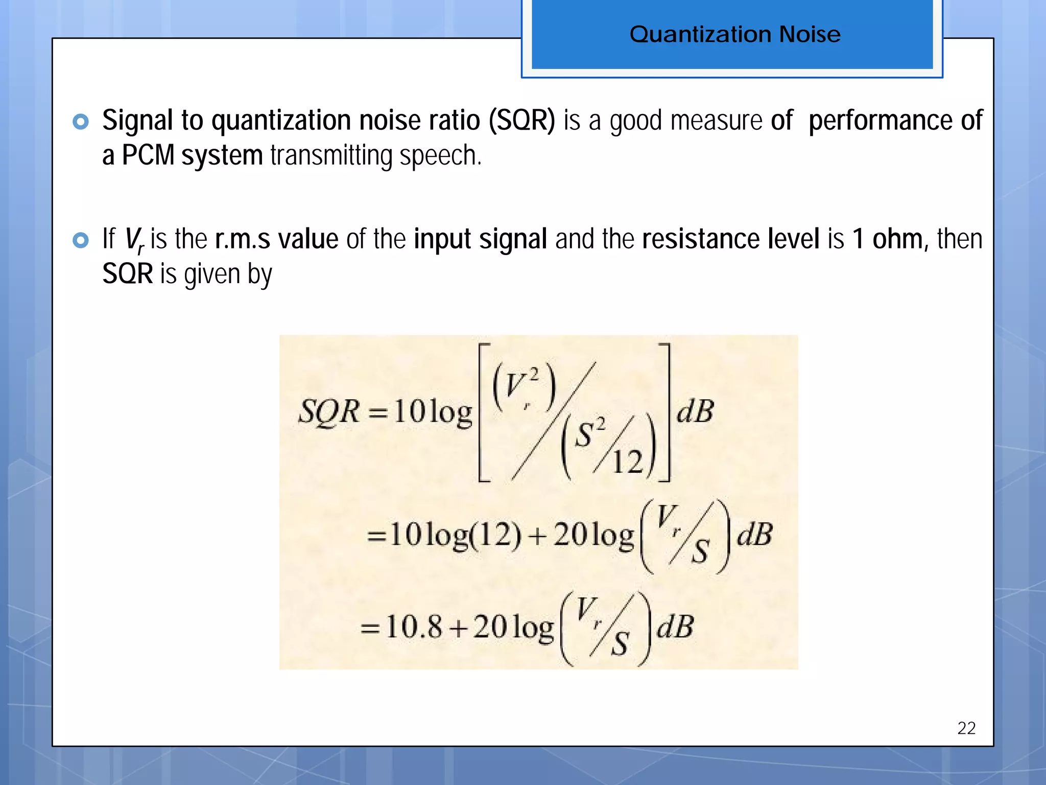
Introduces Signal to Quantization Noise Ratio (SQR) as a performance measure for PCM systems.
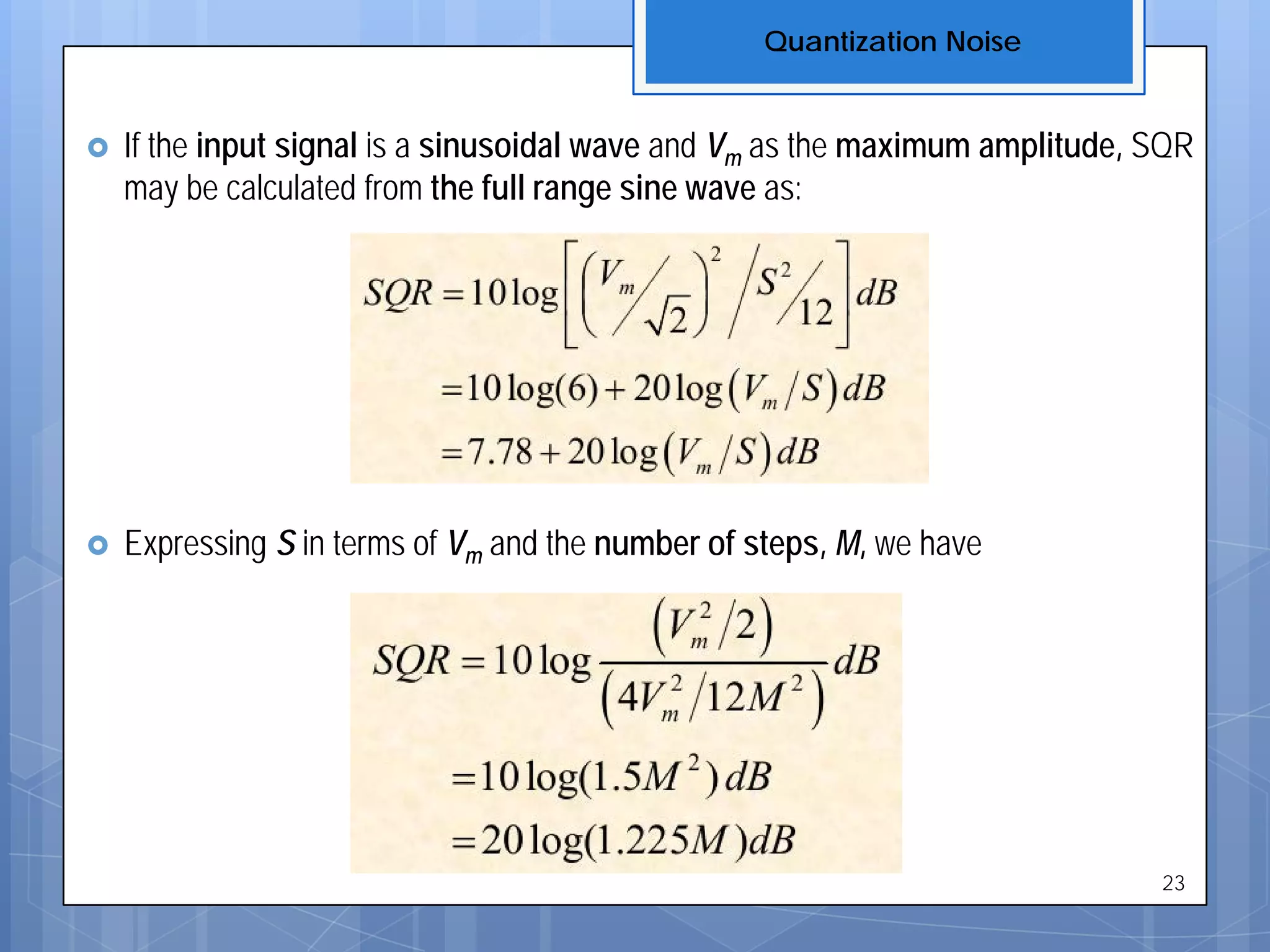
Defines a method to calculate SQR for sinusoidal waves, relating quantization error to signal amplitude.
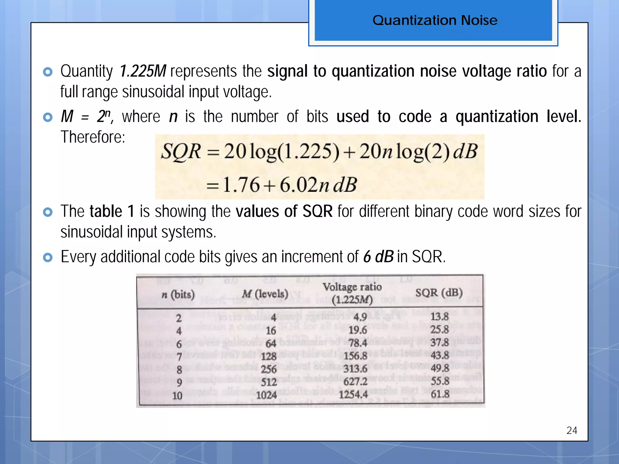
Discusses the relationship between quantization levels and SQR, emphasizing the importance of bit increments.
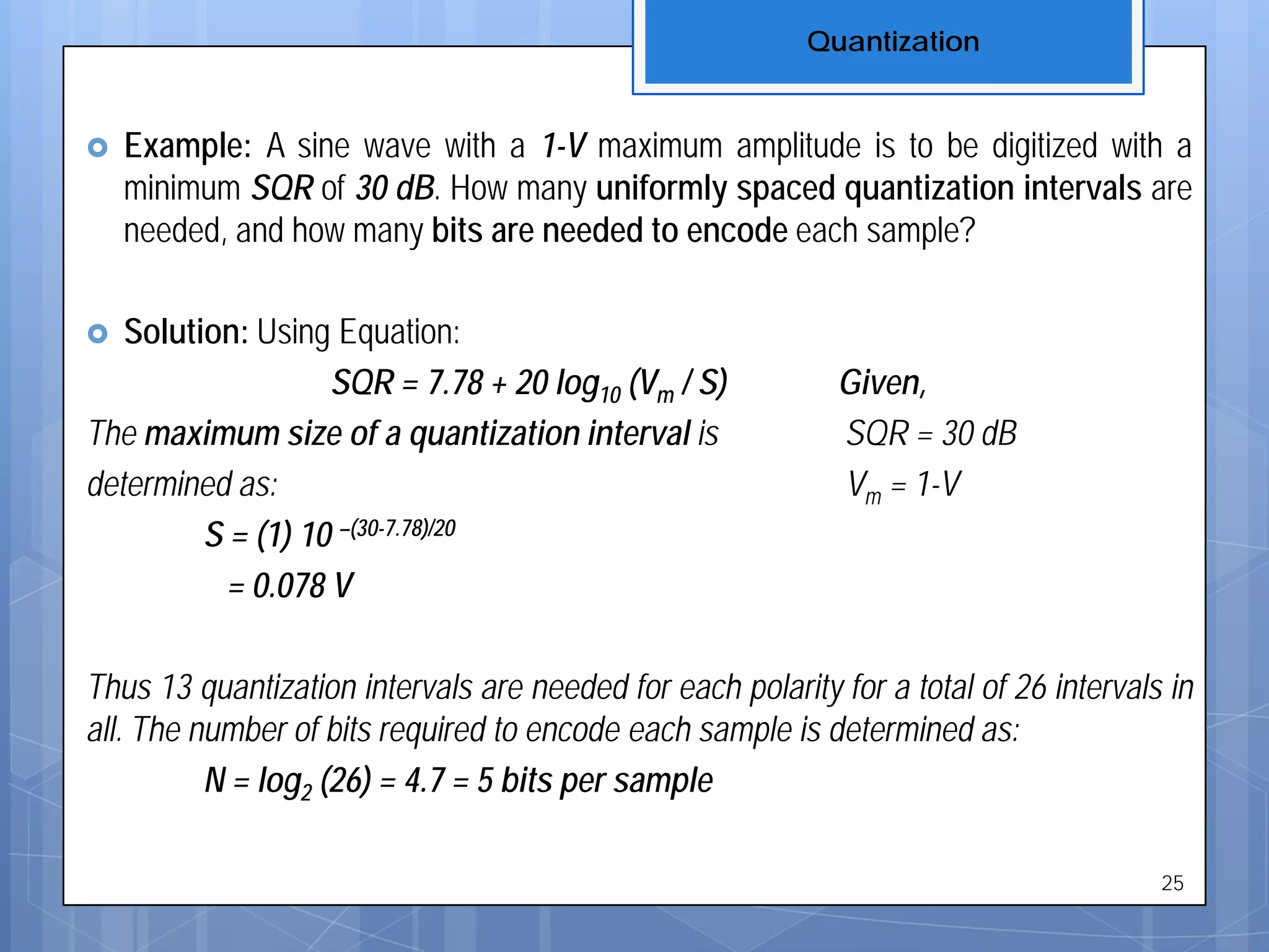
Provides a practical example about calculating required quantization intervals and bits for desired SQR.
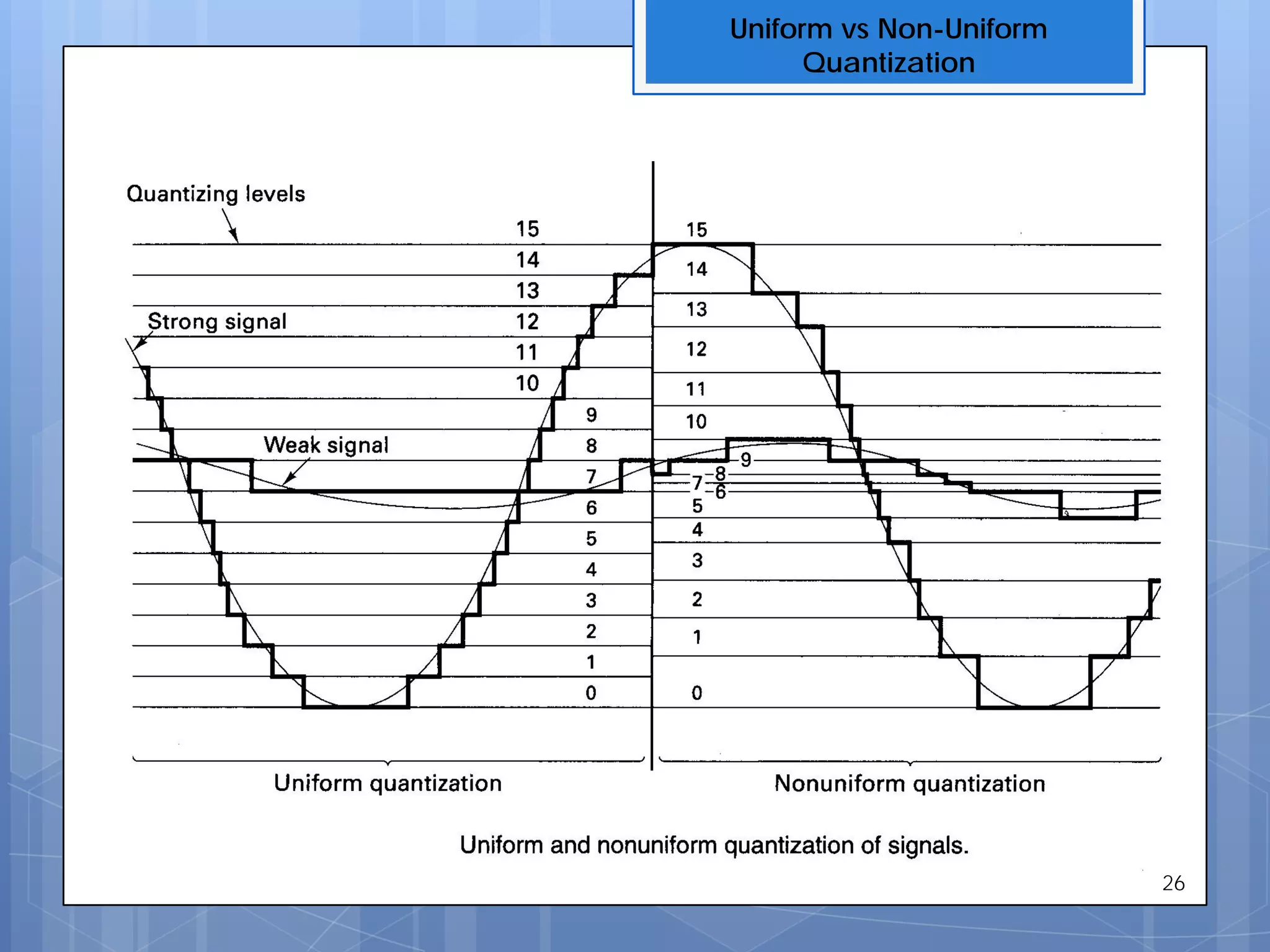
Introduces uniform vs non-uniform quantization techniques and their applications in signal processing.
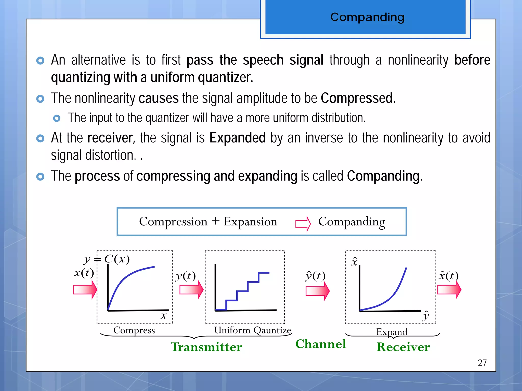
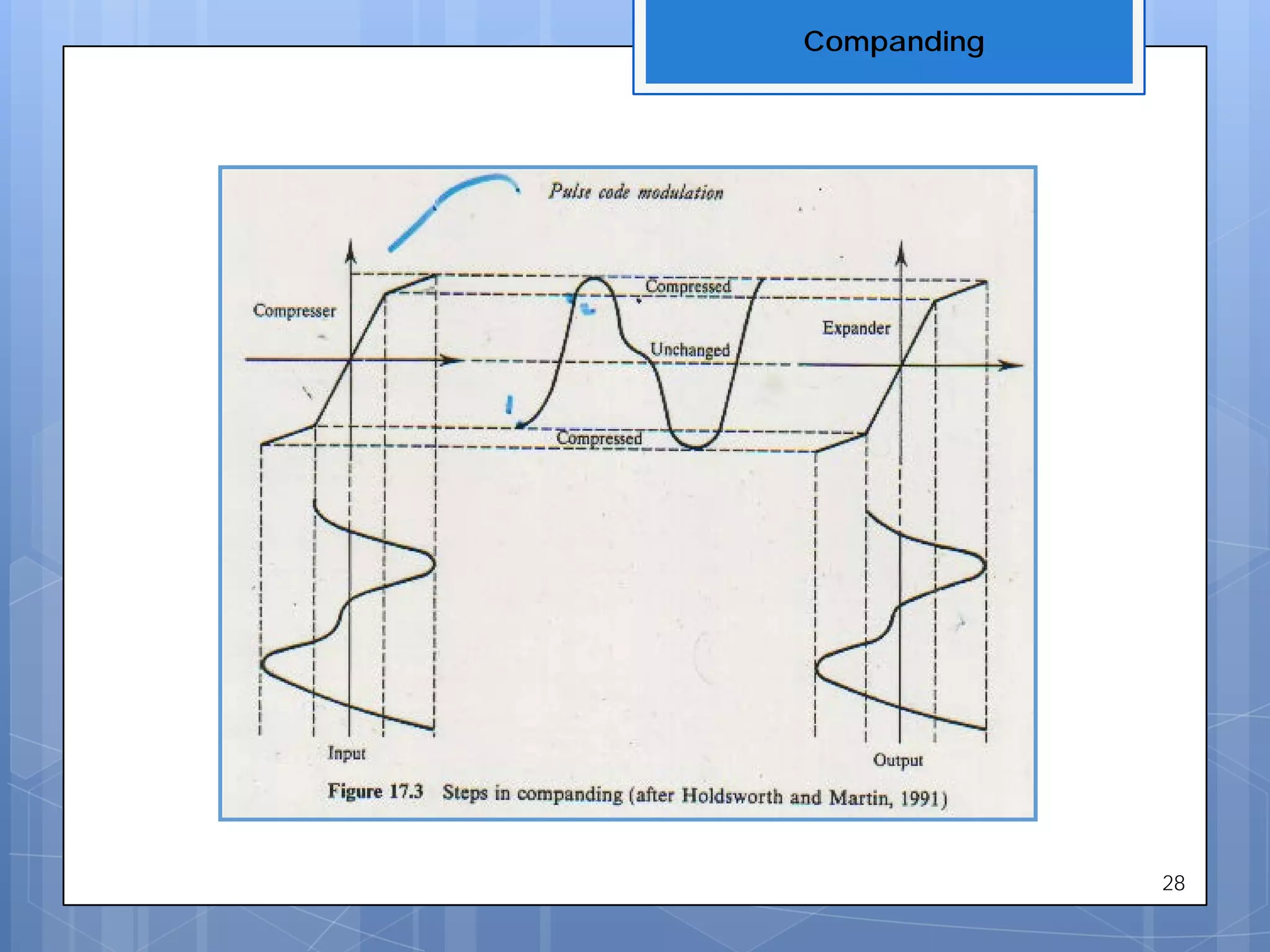
Describes the process of companding—compressing and expanding signals to optimize quantization performance.
Continues discussing companding and its impact on signal processing quality and noise ratios.
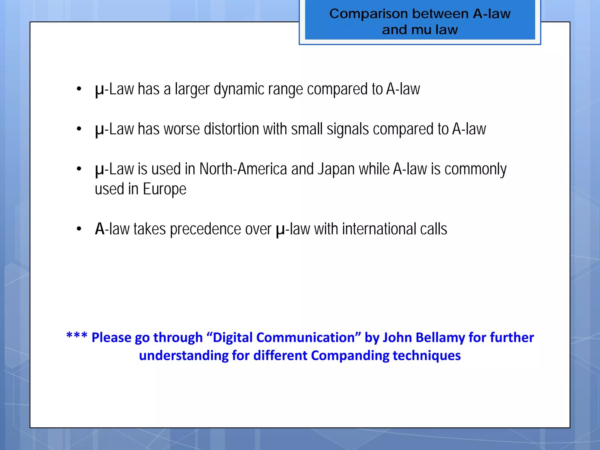
Compares µ-law and A-law companding techniques and their regional applications in telecommunication systems.
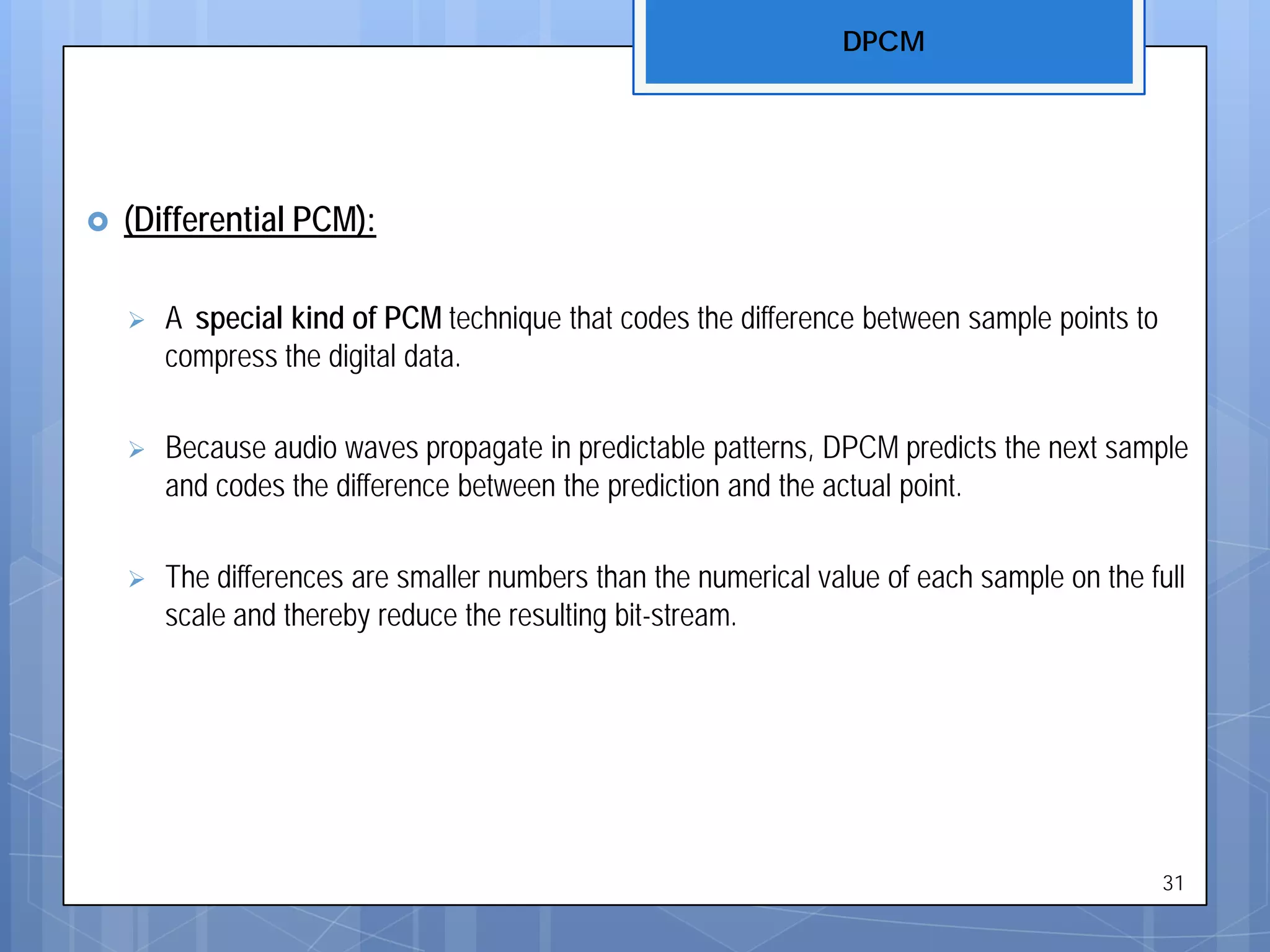
Introduces DPCM, explaining how it reduces data by encoding differences between sample points.
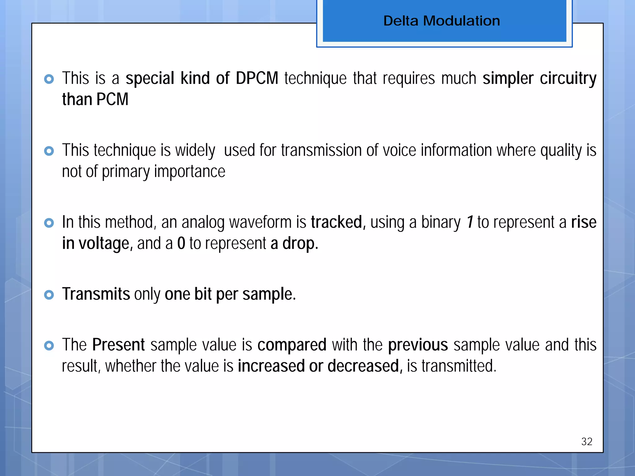
Explains Delta Modulation, focusing on the simplicity of circuitry and its efficiency in voice data transmission.
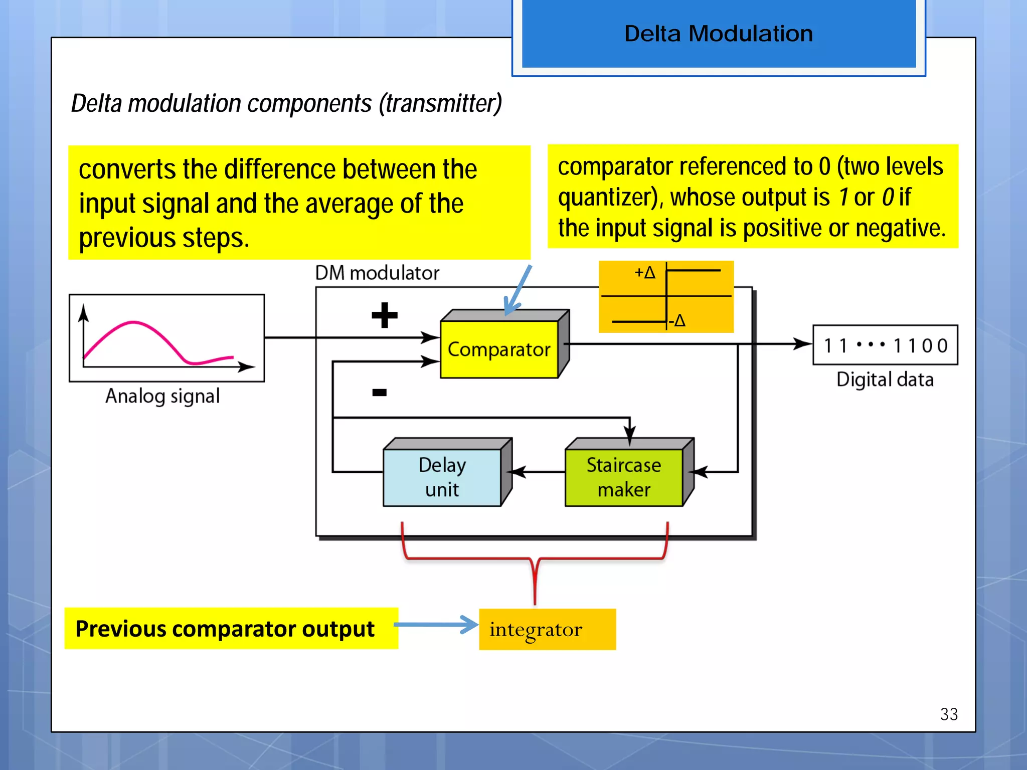
Describes the transmitter components necessary for Delta Modulation, outlining its method of operation.
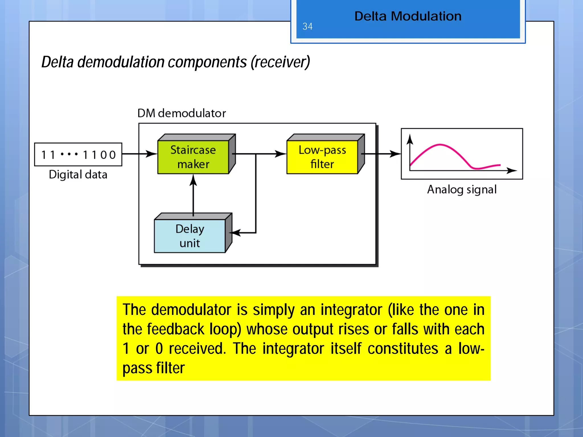
Illustrates the basic demodulation process used in Delta Modulation to reconstruct the transmitted signal.
Discusses potential distortions in Delta Modulation, including slope overload and granular noise and their solutions.
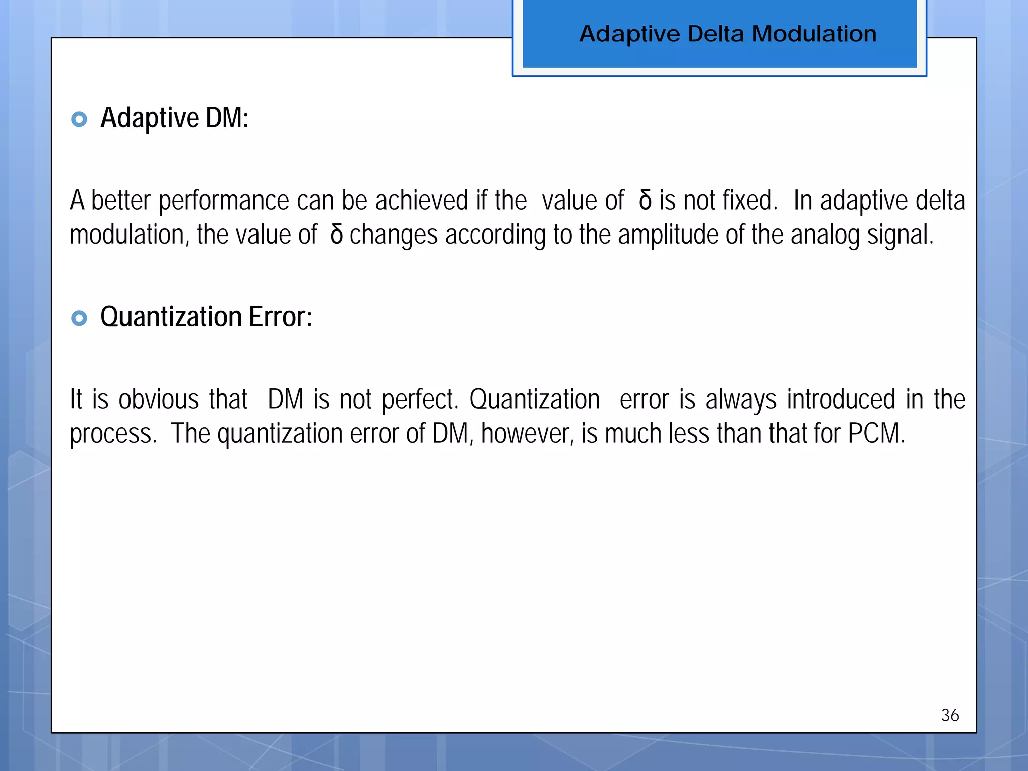
Presents Adaptive Delta Modulation, highlighting its ability to adjust step size based on signal amplitude.
Concludes the presentation, summarizing key technologies and approaches in telecommunications engineering.


![[BDD 2025 - Mobile Development] Mobile Engineer and Software Engineer: Are we...](https://cdn.slidesharecdn.com/ss_thumbnails/md-mobileengineerandsoftwareengineerarewestillrelevantsidiqpermana-251127010650-55224ef1-thumbnail.jpg?width=640&height=640&fit=bounds)
![[DevFest Strasbourg 2025] - NodeJs Can do that !!](https://cdn.slidesharecdn.com/ss_thumbnails/devfeststrasbourg2025-nodejscandothat-251127142731-da65b6fd-thumbnail.jpg?width=640&height=640&fit=bounds)
![[BDD 2025 - Full-Stack Development] Digital Accessibility: Why Developers nee...](https://cdn.slidesharecdn.com/ss_thumbnails/fs-digitalaccessibilitywhydevelopersneedtoknowandcarein2025-251127011019-0674441d-thumbnail.jpg?width=640&height=640&fit=bounds)


![[BDD 2025 - Full-Stack Development] The Modern Stack: Building Web & AI Appli...](https://cdn.slidesharecdn.com/ss_thumbnails/fs-themodernstackbuildingwebaiapplicationswithserverless-251124030844-388cf04f-thumbnail.jpg?width=640&height=640&fit=bounds)


![[BDD 2025 - Mobile Development] Exploring Apple’s On-Device FoundationModels](https://cdn.slidesharecdn.com/ss_thumbnails/md-exploringappleson-devicefoundationmodels-251124030840-d690542c-thumbnail.jpg?width=640&height=640&fit=bounds)


![[BDD 2025 - Full-Stack Development] PHP in AI Age: The Laravel Way. (Rizqy Hi...](https://cdn.slidesharecdn.com/ss_thumbnails/fs-phpinaiagethelaravelway-251125012602-ef9d330e-thumbnail.jpg?width=640&height=640&fit=bounds)
![[BDD 2025 - Artificial Intelligence] AI for the Underdogs: Innovation for Sma...](https://cdn.slidesharecdn.com/ss_thumbnails/ai-aifortheunderdogsinnovationforsmallbusinesses-251124030839-72a599a4-thumbnail.jpg?width=640&height=640&fit=bounds)


