This document discusses one dimensional transient heat conduction. It introduces the full unsteady heat conduction equation and describes how it can be used to model time-varying temperature changes, as in heat treating processes. The lumped capacity assumption is described, where the temperature inside a solid is assumed constant and equal to the surface temperature. An example problem is presented of a metal piece cooling in air after forming. The general solution of the ordinary differential equation for this problem is given. Dimensionless numbers like the Biot number and Fourier number are also defined, with the Biot number representing the ratio of external to internal heat transfer resistance.

1. Heat and mass transfer One Dimensional Transient Heat Conduction
Yashawantha K M, Dept. of Marine Engineering, SIT, Mangaluru Page 1
ONE DIMENSIONAL TRANSIENT HEAT CONDUCTION
Introduction
To this point, we have considered conductive heat transfer problems in which the
temperatures are independent of time. In many applications, however, the temperatures are
varying with time, and we require the understanding of the complete time history of the
temperature variation.
For example, in metallurgy, the heat treating process can be controlled to directly affect
the characteristics of the processed materials. Annealing (slow cool) can soften metals and
improve ductility. On the other hand, quenching (rapid cool) can harden the strain boundary and
increase strength. In order to characterize this transient behavior, the full unsteady equation is
needed:
where is the thermal diffusivity. Without any heat generation and considering
spatial variation of temperature only in x-direction, the above equation reduces to:
For the solution of equation, we need two boundary conditions in x-direction and one initial
condition. Boundary conditions, as the name implies, are frequently specified along the physical
boundary of an object; they can, however, also be internal – e.g. a known temperature gradient at
an internal line of symmetry.
The simplest situation in an unsteady heat transfer process is to use the lumped capacity
assumption, wherein we neglect the temperature distribution inside the solid and only deal with
the heat transfer between the solid and the ambient fluids. In other words, we are assuming that
the temperature inside the solid is constant and is equal to the surface temperature.
The solid object shown in figure is a metal piece which is being cooled in air after hot
forming. Thermal energy is leaving the object from all elements of the surface, and this is shown
for simplicity by a single arrow.
The first law of thermodynamics applied to this problem is
t
T
k
g
q
z
T
y
T
x
T
∂
∂
=+
∂
∂
+
∂
∂
+
∂
∂
α
1
2
2
2
2
2
2
p
c
k
ρ
α =
t
T
x
T
∂
∂
=
∂
∂
α
1
2
2
)(
∞
−= TT
s
hAQ
o
T

2. Heat and mass transfer One Dimensional Transient Heat Conduction
Yashawantha K M, Dept. of Marine Engineering, SIT, Mangaluru Page 2
[Heat out of the object during time dt] = [decrease of internal thermal energy of
object during time dt]
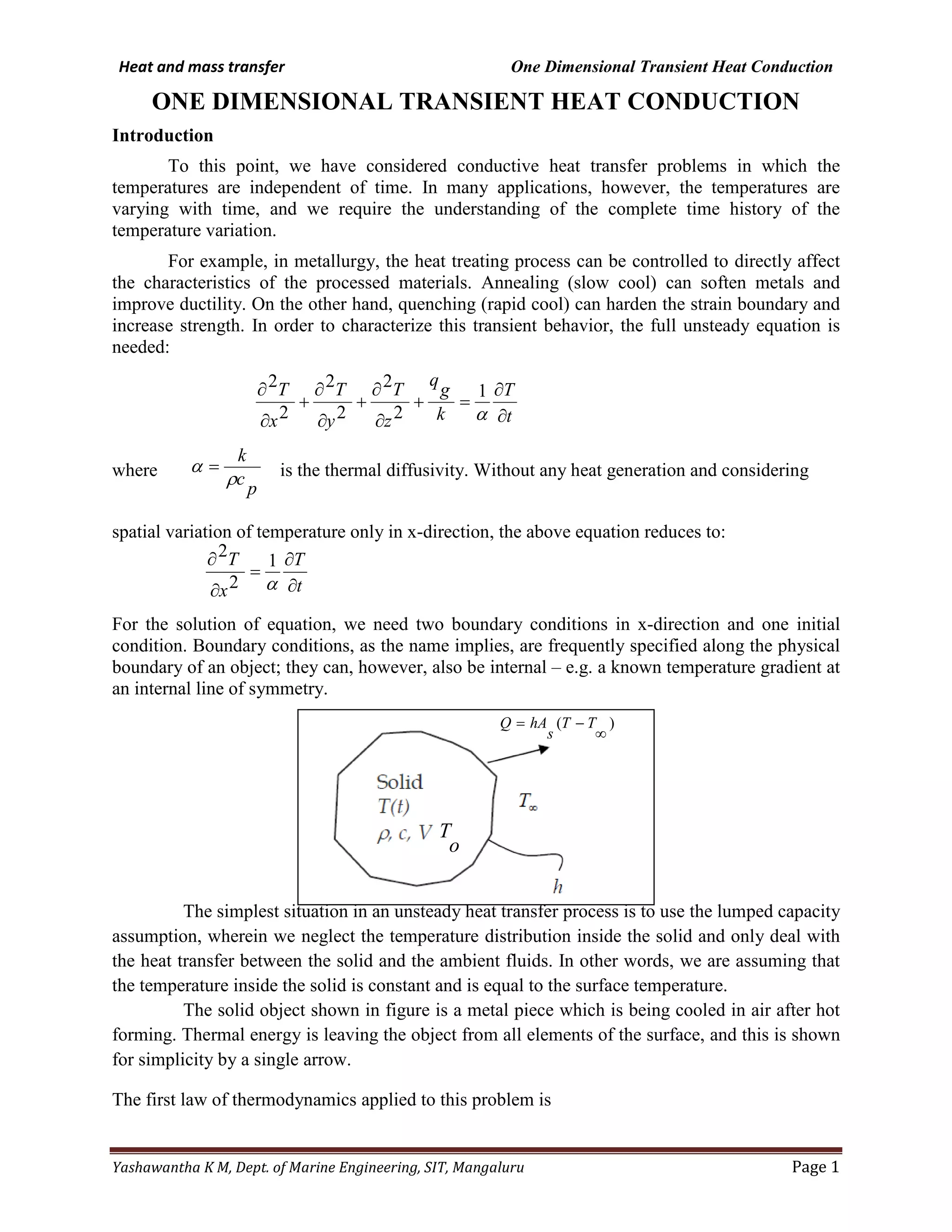
Let consider that a solid f arbitrary shape volume v, total surface area As, thermal conductivity ks,
density ρ , specific heat c. uniform temperature To is suddenly immersed at the time t=0 in a well stirred
fluid which is kept at a uniform temperature
∞
T as shown in figure
The above equation is an ordinal differential equation for the temperature θ (t) and its
general solution given as,
By boundary condition,
(Refer HMTDB Page No 58)
dt
dT
VcTTh
s
A ρ=−
∞
)(
dt
dT
TT
Vc
h
s
A
=−
∞
)(
ρ
)( TT
Vc
h
s
A
dt
dT
−
∞
−=
ρ
)(
∞
−= TT
Vc
h
s
A
dt
dT
ρ
0)( =
∞
−− TT
Vc
h
s
A
dt
dT
ρ
Vc
h
s
A
m
ρ
=
0)( =
∞
−− TTm
dt
dT θ=
∞
−TT
dt
d
dt
dT θ
=0=− θ
θ
m
dt
d
mtCet −=)(θ
0==
∞
− tat
o
T
o
T θ
Co=θ
mtet o
−=θθ )(
mte
o
t −=
θ
θ )(
mte
T
o
T
TT
−=
∞
−
∞
−

3. Heat and mass transfer One Dimensional Transient Heat Conduction
Yashawantha K M, Dept. of Marine Engineering, SIT, Mangaluru Page 3
Biot number
The Biot number is dimensionless, and it can be thought of as the ratio
Whenever the Biot number is small, the internal temperature gradients are also small and
a transient problem can be treated by the “lumped thermal capacity” approach. The lumped
capacity assumption implies that the object for analysis is considered to have a single mass-
averaged temperature.
In general, a characteristic length scale may be obtained by dividing the volume of the
solid by its surface area
Using this method to determine the characteristic length scale, the corresponding Biot
number may be evaluated for objects of any shape, for example a plate, a cylinder, or a sphere.
As a thumb rule, if the Biot number turns out to be less than 0.1, lumped capacity assumption is
applied.a
Physical significance of the Biot number is,
This is the ratio of the heat transfer coefficient for convection at the surface of solid to the
specific conductance of the solid. Hence the assumption of uniform temperature within the solid
is much larger than the heat transfer coefficient for convection.
Fourier number
Fourier number is a dimensionless time can be obtained by multiplying the dimensional time by
the thermal diffusivity and dividing by the square of the characteristic length.
Dimensionless time
(Refer HMTDB Page No 58)
flowheatexternaltoresistance
flowheatinternaltoResistance
=Bi
s
k
Lh
=Bi
s
A
V
=L
L
s
k
h
=Bi
2L
t
Fo
α
=
FoBi
e
T
o
T
TT −
=
∞
−
∞
−

4. Heat and mass transfer One Dimensional Transient Heat Conduction
Yashawantha K M, Dept. of Marine Engineering, SIT, Mangaluru Page 4
REFERENCES
1. Heat transfer-A basic approach, Ozisik, Tata McGraw Hill, 2002
2. Pradeep Dutta, “HEAT AND MASS TRANSFER”, Web based course material under the
NPTEL, Phase 1, 2006.
3. Heat and Mass Transfer Data Book, C.P Kothandarman , S Subramanyan, new age
international publishers ,2010, 7th
edition
4. Fundamental of Heat and Mass transfer, M Thirumaleshwar,Pearson,2013