Two dimension steady state heat comduction.pptx

1. Heat conduction is the transfer of internal thermal energy by the collisions of
microscopic particles and movement of electrons within a body. The microscopic
particles in the heat conduction can be molecules, atoms, and electrons.
Internal energy includes kinematic and potential energy of microscopic particles.
 Heat Conduction
 Cordinate system
Two dimensional system
Problems for only one coordinate direction are grossly oversimplified in many cases.It
is necessary to account for multidimensional effects. Temperature gradients exist
along a two coordinate.

2. 2
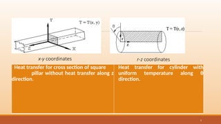
Heat transfer for cross section of square
pillar without heat transfer along z
direction.
Heat transfer for cylinder with
uniform temperature along θ
direction.
x-y coordinates r-z coordinates

3. 3
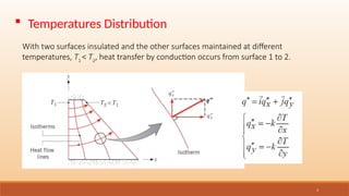
With two surfaces insulated and the other surfaces maintained at different
temperatures, T1
< T2
, heat transfer by conduction occurs from surface 1 to 2.
 Temperatures Distribution

4. 4
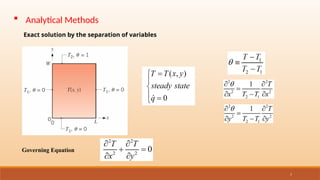
• Analytical method: finding an exact mathematical solution
• Graphical Method: Providing only approximate results at
discrete points
• Numerical method: Providing only aproximate results at
discrete points
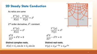
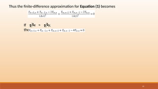
For steady state two dimensional heat conduction with no heat generation, the Laplace
equation applied & Solution of laplace equation is given by following three method i.e

5. 5
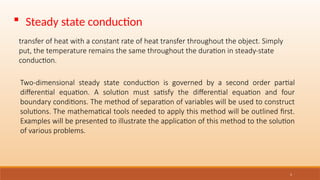
 Steady state conduction
transfer of heat with a constant rate of heat transfer throughout the object. Simply
put, the temperature remains the same throughout the duration in steady-state
conduction.
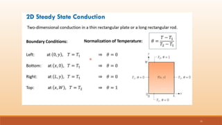
Two-dimensional steady state conduction is governed by a second order partial
differential equation. A solution must satisfy the differential equation and four
boundary conditions. The method of separation of variables will be used to construct
solutions. The mathematical tools needed to apply this method will be outlined first.
Examples will be presented to illustrate the application of this method to the solution
of various problems.

6. 6
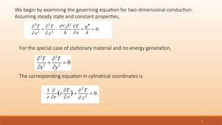
We begin by examining the governing equation for two-dimensional conduction.
Assuming steady state and constant properties,
For the special case of stationary material and no energy generation,
The corresponding equation in cylindrical coordinates is

7. 7
 Analytical Methods
Exact solution by the separation of variables
Governing Equation

8. 8
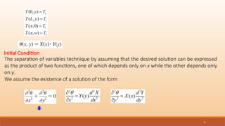
The separation of variables technique by assuming that the desired solution can be expressed
as the product of two functions, one of which depends only on x while the other depends only
on y.
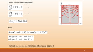
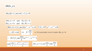
We assume the existence of a solution of the form
Initial Condition

9. 9

10. 10
To find C1, C2, C3, C4, initial conditions are applied
General solution for each equation
Now,

11. 11

12. 12

13. 13

14. 14
n = 0 is precluded, since it implies θ(x, y) = 0

15. 15
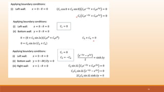
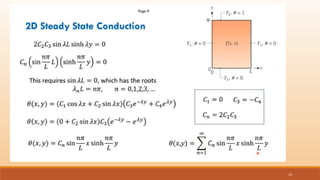
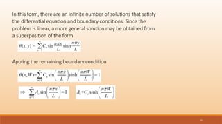
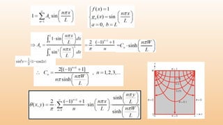
In this form, there are an infinite number of solutions that satisfy
the differential equation and boundary conditions. Since the
problem is linear, a more general solution may be obtained from
a superposition of the form
Appling the remaining boundary condition

16. 16
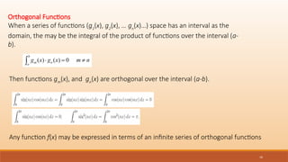
Orthogonal Functions
When a series of functions (g1
(x), g2
(x), … gn
(x)…) space has an interval as the
domain, the may be the integral of the product of functions over the interval (a-
b).
Then functions gm
(x), and gn
(x) are orthogonal over the interval (a-b).
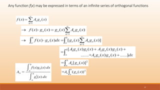
Any function f(x) may be expressed in terms of an infinite series of orthogonal functions

17. 17
Any function f(x) may be expressed in terms of an infinite series of orthogonal functions

19. 19
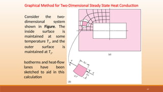
Graphical Method for Two-Dimensional Steady State Heat Conduction
Consider the two-
dimensional system
shown in Figure. The
inside surface is
maintained at some
temperature T1, and the
outer surface is
maintained at T2.
Isotherms and heat-flow
lanes have been
sketched to aid in this
calculation

20. 20
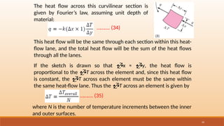
The heat flow across this curvilinear section is
given by Fourier’s law, assuming unit depth of
material:
………. (34)
This heat flow will be the same through each section within this heat-
flow lane, and the total heat flow will be the sum of the heat flows
through all the lanes.
If the sketch is drawn so that x ≈ y, the heat flow is
proportional to the T across the element and, since this heat flow
is constant, the T across each element must be the same within
the same heat-flow lane. Thus the T across an element is given by
………. (35)
where N is the number of temperature increments between the inner
and outer surfaces.

21. 21
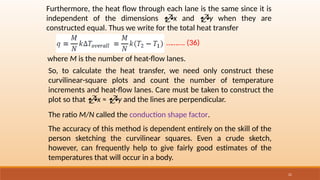
Furthermore, the heat flow through each lane is the same since it is
independent of the dimensions x and y when they are
constructed equal. Thus we write for the total heat transfer
………. (36)
where M is the number of heat-flow lanes.
So, to calculate the heat transfer, we need only construct these
curvilinear-square plots and count the number of temperature
increments and heat-flow lanes. Care must be taken to construct the
plot so that x ≈ y and the lines are perpendicular.
The ratio M/N called the conduction shape factor.
The accuracy of this method is dependent entirely on the skill of the
person sketching the curvilinear squares. Even a crude sketch,
however, can frequently help to give fairly good estimates of the
temperatures that will occur in a body.

22. 22
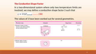
The Conduction Shape Factor
In a two-dimensional system where only two temperature limits are
involved, we may define a conduction shape factor S such that
………. (36)
The values of S have been worked out for several geometries.

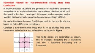
23. Numerical Method for Two-Dimensional Steady State Heat
Conduction
In many practical situations the geometry or boundary conditions
are such that an analytical solution has not been obtained at all, or if
the solution has been developed, it involves such a complex series
solution that numerical evaluation becomes exceedingly difficult.
For such situations the most fruitful approach to the problem is one
based on finite-difference techniques.
Consider a two-dimensional body that is to be divided into equal
increments in both the x and y directions, as shown in Figure.
The nodal points are designated as shown,
the m locations indicating the x increment
and the n locations indicating the y
increment.

24. 24
The temperature gradients may be written as follows:

25. 25
Thus the finite-difference approximation for Equation (1) becomes
If x ≈ y,
then

26. 26
Unsteady state heat transfer refers to the process in which the temperature of a system or an
object changes as a function of time. This is in contrast to steady-state heat transfer, in which
the system’s or object’s temperature remains constant over time. This type of heat transfer can
happen in different forms, such as conduction, convection, and radiation. It occurs in various
systems, including solid materials, fluids, and gases. The heat transfer rate in an unsteady state
is directly proportional to the rate of temperature change. This means that the heat transfer
rate is not constant and can vary over time. It’s an important aspect in the design and
optimization of thermal systems, and understanding this process is crucial in many research
areas, such as combustion, electronics, and aerospace.
Unsteady State Heat Conduction
(mass and energy in the system are changing with time (not constant).)

27. Types of Unsteady State Heat Transfer
There are three main types of unsteady state heat transfer:
 One-dimensional heat conduction: This type of heat transfer occurs in materials where heat
is transferred in only one direction. An example of this would be heat transfer through a
metal rod.
 Transient convection: This heat transfer occurs in fluids, such as liquids and gases, and is
characterized by the movement of the fluid and the associated heat transfer. An example of
transient convection would be heat transfer in a fluid flowing through a pipe.
 Radiative heat transfer: This heat transfer occurs through the emission and absorption of
electromagnetic radiation. An example of this would be heat transfer through a window.
Additionally, it’s also possible to have a combination of these types of heat transfer in a system,
for example, conduction through a solid material and convection through a fluid, known as
unsteady state conduction-convection heat transfer.

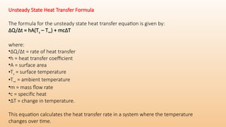
28. Unsteady State Heat Transfer Formula
The formula for the unsteady state heat transfer equation is given by:
ΔQ/Δt = hA(Ts – T∞) + mcΔT
where:
•ΔQ/Δt = rate of heat transfer
•h = heat transfer coefficient
•A = surface area
•Ts = surface temperature
•T∞ = ambient temperature
•m = mass flow rate
•c = specific heat
•ΔT = change in temperature.
This equation calculates the heat transfer rate in a system where the temperature
changes over time.

29. Applications of Unsteady State Heat Transfer
Unsteady state heat transfer has a wide range of applications, including:
1.Industrial processes commonly design heat exchangers, boilers, and reactors.
2.Automotive engineering: It is used to analyse cooling systems in automobiles, which are
typically subjected to rapid changes in temperature and flow conditions.
3.Aerospace engineering analyses the thermal performance of aerospace vehicles such as
missiles and spacecraft operating in rapidly changing environments.
4.Energy systems: It is used to model the performance of solar thermal, geothermal, and
other renewable energy systems subject to changing temperature and flow conditions.
5.Building heating and cooling: It is used to model the performance of heating, ventilation,
and air conditioning (HVAC) systems in buildings, which are typically subject to changing
temperature and flow conditions.
6.Food processing: It is used in the food processing industry to model the heat transfer
during the cooking, drying and freezing processes.
7.Biomedical Engineering: It is used to analyse temperature changes in the human body
during medical procedures such as hyperthermia treatment for cancer.

30. Limitations of Unsteady State Heat Transfer
There are several limitations of unsteady state heat transfer, including:
1.Complexity: Unsteady-state heat transfer problems are generally more complex than steady-
state problems due to the need to track the changing temperature and flow conditions over
time.
2.Solution methods: A limited number of analytical solutions are available for unsteady state
heat transfer problems, and most problems require numerical solution methods.
3.Data requirements: Unsteady-state heat transfer problems typically require more detailed
information about the initial and boundary conditions than steady-state problems.
4.Time-dependent: The heat transfer rate, temperature, and other parameters change with
time, so it requires more data points to model the system accurately.
5.Difficulties in measuring: Measuring the unsteady heat transfer coefficient and other
parameters is difficult, and it requires specialized techniques.
6.Modelling assumptions: Some unsteady state heat transfer problems may require simplifying
assumptions, such as lumped system analysis, which may not be valid for all situations.
7.Thermal mass effect: The thermal mass effect, which is the ability of an object to store
thermal energy, can cause delays in temperature changes in some cases.

31. 31
Any question ??
Thank you