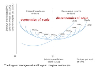
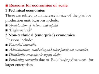
This document discusses production and costs in both the short-run and long-run. In the short-run, at least one factor of production is fixed, while in the long-run all factors are variable. The factors of production are land, labor, capital, and entrepreneurship. Laws of returns to scale describe how output responds to changing variable inputs. Short-run costs include total, fixed, and variable costs. Long-run average costs depend on whether there are increasing, constant, or decreasing returns to scale. Economies of scale from specialization, bulk purchasing, and other factors can lower long-run average costs.

1. Production and Cost

2. • Short-run time period (SR) is that period of time in which
at least one factor of production is fixed and cannot be
changed. SR could vary across firms
• Long-run time period (LR) is that period of time in which
all factors of production can be varied. LR could also
vary across firms.
The factors of production
• Inputs required to produce a particular product such as
land, labour, capital and enterprise.
• ■ Land – ‘all the free gifts of nature’ which could be
Renewable resources (wind, water and other power sources)
which can be reproduced.
• Non-renewable resources (coal, oil) which cannot be reused.
• Land is immovable.

3. ■ Labour – includes:
1. the number of people available for the production
of goods or services,
2. their physical and intellectual abilities.
• The labour force - = No employed + No Unemployed
• Organizing work to guarantee higher output yields:
• ‘Division of labour’ or ‘specialisation’ - refers to the
way in which economic activities are broken down
into their various component parts so that each
worker performs only a small part of the entire
operation.
• ■ Capital - man-made asset used in support of the
production of further goods and services.

4. Note: “use” determines whether or not an asset is
regarded as capital.
Fixed capital - used time and again in the production
process (factory buildings, or educational buildings)
Circulating capital - used once which consists of raw
materials and other intermediate inputs into the
production process.
• ■ Enterprise - also referred to as entrepreneurship.
• The entrepreneur is seen as performing two important
roles:
• ■ hiring and combining factors of production;
• ■ risk-taking by producing goods and services
anticipation of demand which may, or may not,
materialise.

5. Combining factors of production: the laws of
returns
• ■ Total product (TP). This is simply the total output
a firm produces within a given period of time. For
example, the total product of a particular firm might
be 1,000 units per week.
• ■ Average product (AP). This is usually measured in
relation to a particular factor of production, such as
labour or capital.
• Average product of labour (APL)= Total
product/Total labour input
• ■ Marginal product (MP). Marginal product is the
change in total product when one more unit of the
factor is used.
Marginal product of labour (MPL) =

6. ■ Law of variable proportions
• applies to the short-run time period when at least one
factor of production (usually capital) is fixed.
• Increasing returns to the variable factor
• Given a fixed factor, capital
• Output rises more than in proportion to the extra input
of variable factor, and we say that increasing returns have
set in.
• Diminishing returns to the variable factor
• Beyond the optimum proportion of variable to fixed
factor, additional units of the variable factor, here
labour, will be progressively less productive, and we
now say that diminishing returns have set in.

7. Production with OneVariable Input (Labour)
TABLE 1 PRODUCTION WITH ONE VARIABLE INPUT
LABOUR (L)
AMOUNT OF
CAPITAL (K)
TOTAL
PRODUCT
(TP)
AVERAGE
PRODUCT (TP/L)
MARGINAL PRODUCT (MP)
( q/ L)
0 10 0 — —
1 10 10 10 10
2 10 30 15 20
3 10 60 20 30
4 10 80 20 20
5 10 95 19 15
6 10 108 18 13
7 10 112 16 4
8 10 112 14 0
9 10 108 12 -4
10 10 100 10 -8

8. The Slopes of the Product Curve
PRODUCTION WITH
ONE VARIABLE INPUT
Figure (1 of 2)
The total product curve in (a) shows
the output produced for different
amounts of labor input.
The average and marginal products in
(b) can be obtained (using the data in
Table 1) from the total product curve.
At point A in (a), the marginal product
is 20 because the tangent to the total
product curve has a slope of 20.
At point B in (a) the average product
of labor is 20, which is the slope of the
line from the origin to B.
The average product of labor at point
C in (a) is given by the slope of the
line 0C.
20

9. The Slopes of the Product Curve
PRODUCTION WITH
ONE VARIABLE INPUT
Figure (2 of 2)
To the left of point E in (b), the
marginal product is above the average
product and the average is increasing;
to the right of E, the marginal product
is below the average product and the
average is decreasing.
As a result, E represents the point at
which the average and marginal
products are equal, when the average
product reaches its maximum.
At D, when total output is maximized,
the slope of the tangent to the total
product curve is 0, as is the marginal
product.
20

10. Costs of production: short run
• Fixed costs – fixed costs are incurred even when the firm’s output
is zero such as mortgage or rent on premises, is indirectly related to
output. They are therefore sometimes referred to as indirect costs or
overheads.
• Variable costs
• The costs that vary directly with output such as costs of raw
materials and components, wages of labour and so on.
• In the SHORT-RUN, cost can be divided into:
• Total Cost (TC), Total Fixed Cost (TFC) and Total Variable
Cost (TVC)
 Note: Connection between TVC and TP assume L – only variable
factor:
1. Output now on X-axis, labour cost (TVC) now on Y-axis
2. TVC inverse shape of TP.

14. • TFC is a horizontal straight
line.
• However, TVC is usually
drawn as an inverted letter
‘S’, suggesting that
increasing returns to the
variable factor initially mean
that total variable costs rise
relatively slowly with output.
• However, as diminishing
returns set in, the total
variable costs rise at an
increasingly rapid rate with
output.

15. • (AFC) fall continuously
• (MC) curve slopes downwards
initially, with falling marginal
costs the mirror image of
increasing marginal returns
to the variable factor in the
short run
• At output Q1 diminishing
marginal returns set in and
the MC curve begins to rise.
• Note that the ATC curve is the
vertical sum of AFC and AVC
curves and this starts to rise
after output Q3 when the rise in
AVC outweighs the fall in AFC.

16. ■ Costs of production: long run
• In the long run all factors become variable and the firm is able to
change the scale of plant, for example, by moving to a new
production site.
Long-run are series of short-run positions
• There are three possibilities:
 Constant returns to scale – output increases in the same
proportion as the employment of inputs. Average cost of
production remains unaltered so long as factor prices
remain constant.
 Increasing returns to scale – output increases at a greater
rate than the employment of inputs. Average cost of
production falls with constant factor prices.

17.  Decreasing returns to scale – output increases at a slower rate
than the employment of inputs. Average cost of production
increases with constant factor prices.
• When measuring returns to scale we assume (as above) that
all factor inputs are changed in the same proportion, i.e.
maintaining the ratio between factor inputs.
• In reality this might not be the case since at higher output
levels new technologies might become possible.

18. Figure 5.9 The relationship between short- and long-run average cost curves,
increasing returns to scale

19. The long-run average cost and long-run marginal cost curves
economies of scale diseconomies of scale

20. ■ Reasons for economies of scale
1 Technical economies
These are related to an increase in size of the plant or
production unit. Reasons include:
■ Specialisation of labour and capital
■ ‘Engineers’ rule’
2 Non-technical (enterprise) economies
Reasons include:
■ Financial economies.
■ Administrative, marketing and other functional economies.
■ Distributive economies ie supply chain
■ Purchasing economies due to Bulk buying discounts for
larger enterprises.