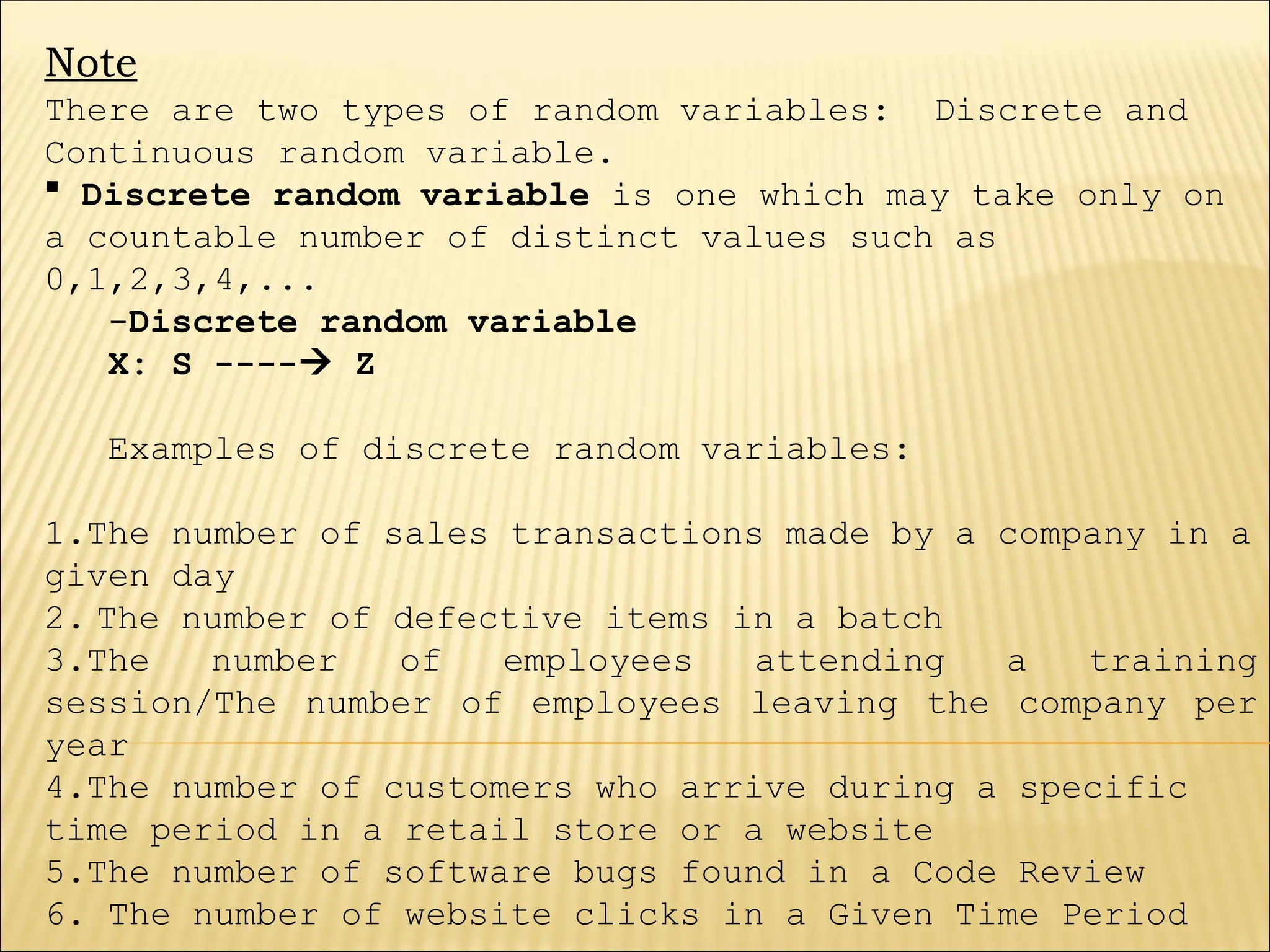
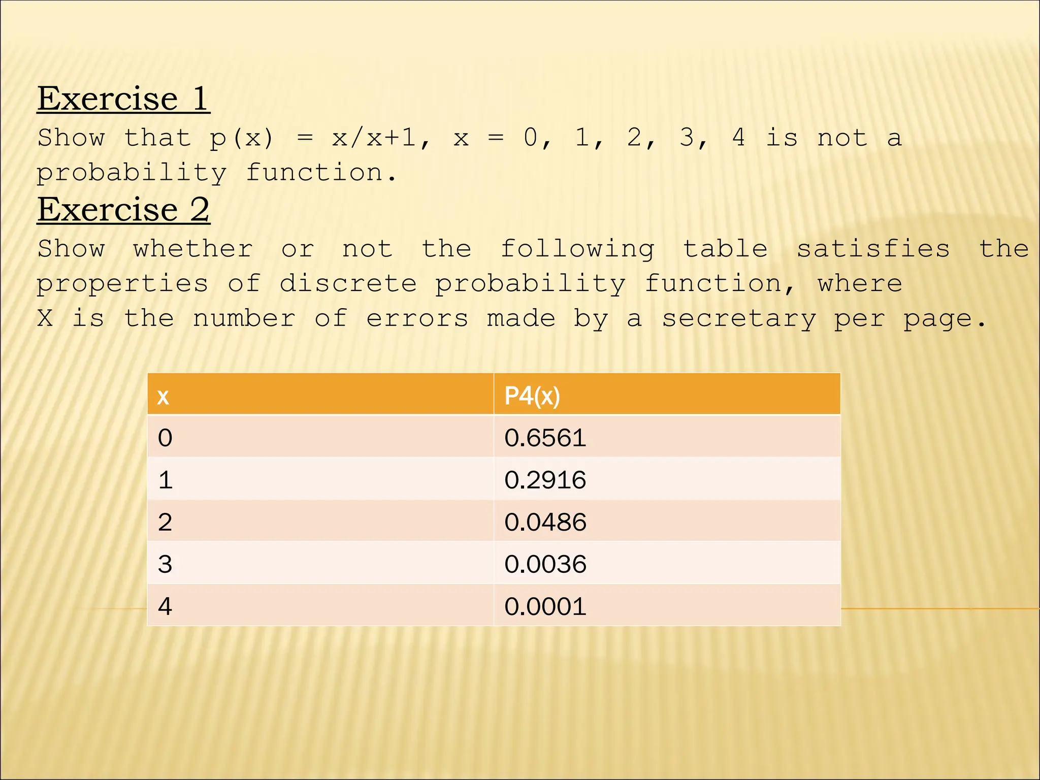
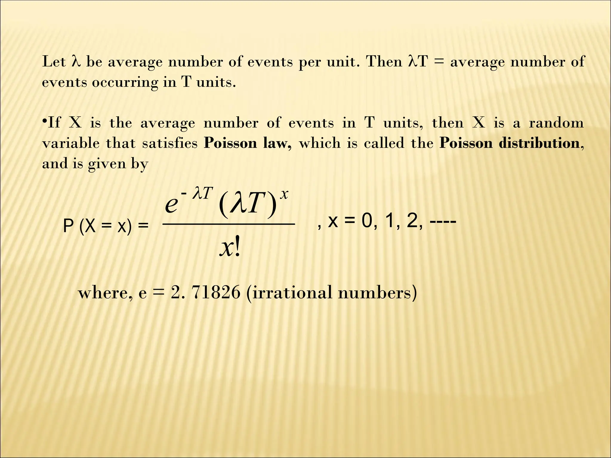
Chapter 1 discusses probability distributions, focusing on random phenomena and the analysis of outcomes from random experiments. It introduces key concepts such as sample space, events, independence of events, random variables, and types of random variables, along with detailed explanations of discrete and continuous random variables. The chapter also covers the definitions and applications of probability functions, expected values, variances, and introduces binomial distributions as examples of discrete probability distributions.

1. CHAPTER 1
PROBABILITY DISTRIBUTION

2.  It is concerned with the analysis of random
phenomena. The outcome of a random event cannot be
determined before it occurs, but it may be any one of
several possible outcomes. The actual outcome is
considered to be determined by chance.
 It is the measure of the likelihood that an event
will occur in a Random Experiment(i.e. Whenever we’re
unsure about the outcome of an event, we can talk
about the probabilities of certain outcomes—how
likely they are).

3.  Experiment: is a trial/process that generates two or
more possible outcomes.
 Sample space/outcome space: The set ALL possible
outcomes of an experiment.
 Event: is any subset of sample space.
Example 1:
Experiment: Toss/Flip a coin once
Sample space: Head, Tail
Event:
Example 2:
Experiment: Toss a coin twice
Sample space: (Head,Head),Head, Tail),(Tail, Head),
(Tail,Tail).
Event:
Experiment: Measuring the time until the bus comes
Sample space: (0, )
Event:

4. Classical definition of probability:
 Let A be an event and S a sample space, then
 P(A)=n(A)/n(S)
Example 1: What is the probability of getting atmost 2
head in tossing a coin twice? Three times?
Example 2: What is the probability that both coins turn
up the same in rolling a die twice? What is the
probability of getting a sum of 12 in this
experiment?
Example 3: What is the probability of drawing an Ace in
a deck of 52 playing cards, when selection is with
replacement? Without replacement?

5.  Two events are independent if and only if the
occurrence of the first event does not have an effect
on the probability of occurrence of the second
event(Events A and B are independent if: knowing
whether A occurred does not change the probability of
B). If two events are not independent, then they are
said to be dependent events.
Example: Let A = the event of drawing number 10 in a
deck of 52 playing cards,
B = the event of drawing number 5
 If A and B are chosen without replacement, are they
independent?
 If A and B are chosen with replacement, are they
independent?
NB: If A and B are independent, then P(AnB)=P(A)P(B)
Exercise: Experiment is rolling a die twice; A = first
die lands 1; B = second die shows larger number than
first die; C = both dice show same number. Are A and B
independent? Are A and C independent?

6. Let A and B be two events:
The conditional probability of an event A is the
probability that the event will occur given the
knowledge that an event B has already occurred. This
probability is written P(A|B), notation for
the probability of A given B.
 P(A|B)= P(AnB)/P(B)
NB: If A and B are independent, then P(A|B)= P(A)
Illustrative example:The weatherman might state that
your area has a probability of rain of 40%. However,
this fact is conditional on many things, such as the
probability of…
 …a cold front coming to your area.
 …rain clouds forming.
 …another front pushing the rain clouds away, etc.

7.  Example: Suppose an individual applying to a college
determines that he has an 80% chance of being
accepted, and he knows that dormitory housing will
only be provided for 60% of all of the accepted
students. The chance of the student being
accepted and receiving dormitory housing is defined
by
P(Accepted and Dormitory Housing) = P(Dormitory
Housing|Accepted)P(Accepted) = (0.60)*(0.80) = 0.48.

8. Random variable
Definition: A random variable is a variable whose
values are determined by all possible outcomes of a
random experiment (i.e., when the value of a variable
is obtained from the outcome of an experiment, that
variable is said to be random variable).
•It is a quantitative result generated from a random
experiment
•It assigns unique numerical values to each of the
outcomes of an experiment.
• It subjects to randomness, and may take on many
numerical values.
•It is a variable whose future values are uncertain.
Notation
a random variable is denoted by X, and its value is
represented by x

9. Examples
1.Toss a coin two times. Let X be number of heads
obtained.
Is X a random variable?
S = sample space = { HH, HT, TH, TT}
n(TT) = 0
n(HT)= n(TH)=1
n(HH)=2
Therefore, X = x, x = 0, 1, 2.
2.Toss a coin 8 times. Let X be number of tails
obtained.
X = x, x = 0, 1, 2, 3, 4, 5, 6, 7,8
outcome TT HT HH
N(outcome),x 0 1 2

10. 3. Let X be number of children of a family in A.A.
X = x, x = 0, 1, 2, 3, 4, ------- K
Where k = maximum number of children
4. Let X be the mark of a student in a particular
exam (out of 100)
X = x, 0 ≤ x ≤ 100. – Infinitely many values
5. Let X be the life length in hrs of an electric
bulb.
X = x, 0 ≤ x ≤ k, where k = max. life length
6. Let X = the market share of the product at a
particular time.
7. Let X= the monthly unemployment figures in Ethiopia
over the last 10 years.
8. Let X= the sales of a particular product at a
particular time.

11. Note
There are two types of random variables: Discrete and
Continuous random variable.
 Discrete random variable is one which may take only on
a countable number of distinct values such as
0,1,2,3,4,...
-Discrete random variable
X: S ---- Z
Examples of discrete random variables:
1.The number of sales transactions made by a company in a
given day
2. The number of defective items in a batch
3.The number of employees attending a training
session/The number of employees leaving the company per
year
4.The number of customers who arrive during a specific
time period in a retail store or a website
5.The number of software bugs found in a Code Review
6. The number of website clicks in a Given Time Period

12. A continuous random variable is a vriable that assigns
any value in an interval
It is the one which takes an infinite number of
possible values
Continuous random variable
X: S------R
Examples of continuous random variables:
1.The total revenue generated by a company from sales can
be modeled as a continuous random variable, as it can take
on any real value within a certain range
2. Time Spent on Customer Service Calls: The time taken to
resolve customer service calls
3. Interest Rate: When dealing with financial instruments
such as bonds or loans, the interest rate can be treated
as a continuous random variable

13. Discrete probability function
Definition: Let X be a discrete random variable
with finite number of values: x1
, x2
, ---- xn.,
and
the corresponding probabilities
p(xi
) = p(X = xi
), i = 1, 2,…,n
Then the function p(xi
) is called the
probability function of X if the following
conditions are satisfied
i) p(xi
)≥ 0 for all x
ii)


n
i
i
x
p
1
)
( = 1

14. Example 1
Check if p(x) = 1/4, x = 0, 1, 2, 3. is a probability
function or not.
Example 2
Suppose a variable X can take the values 1, 2, 3,or 4.
The probabilities associated with each outcome are
described by the following table:
Outcome 1 2 3 4
Probability 0.1 0.3 0.4 0.2

15. Exercise 1
Show that p(x) = x/x+1, x = 0, 1, 2, 3, 4 is not a
probability function.
Exercise 2
Show whether or not the following table satisfies the
properties of discrete probability function, where
X is the number of errors made by a secretary per page.
x P4(x)
0 0.6561
1 0.2916
2 0.0486
3 0.0036
4 0.0001

16. Discrete probability distribution
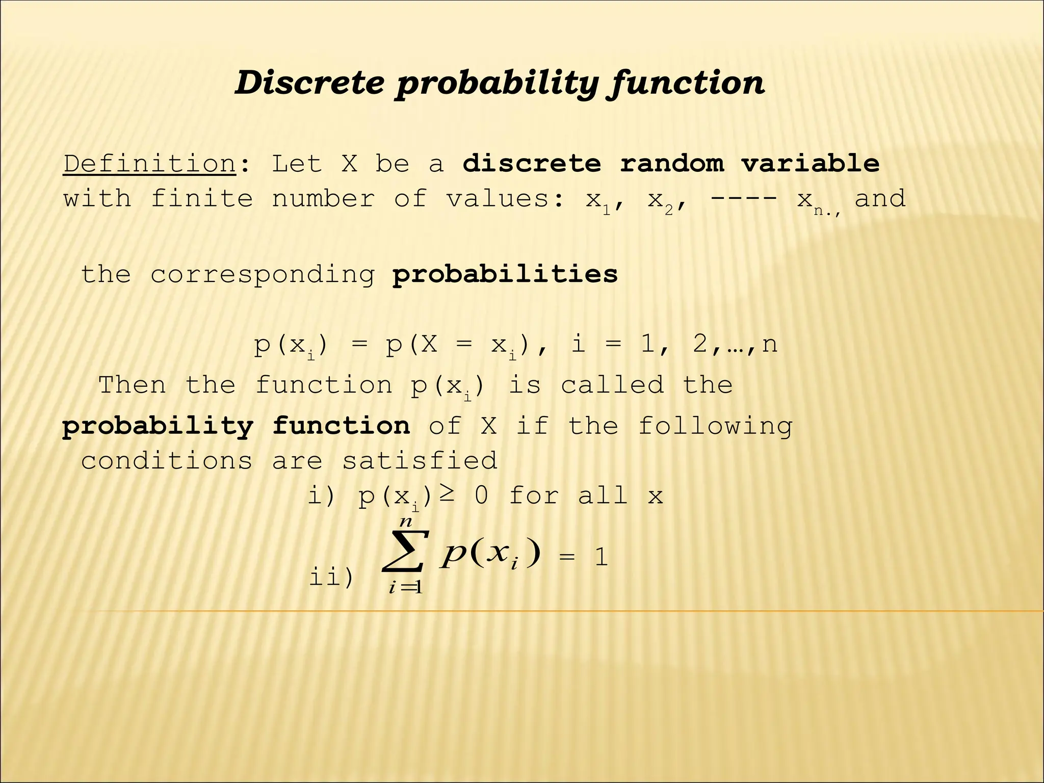
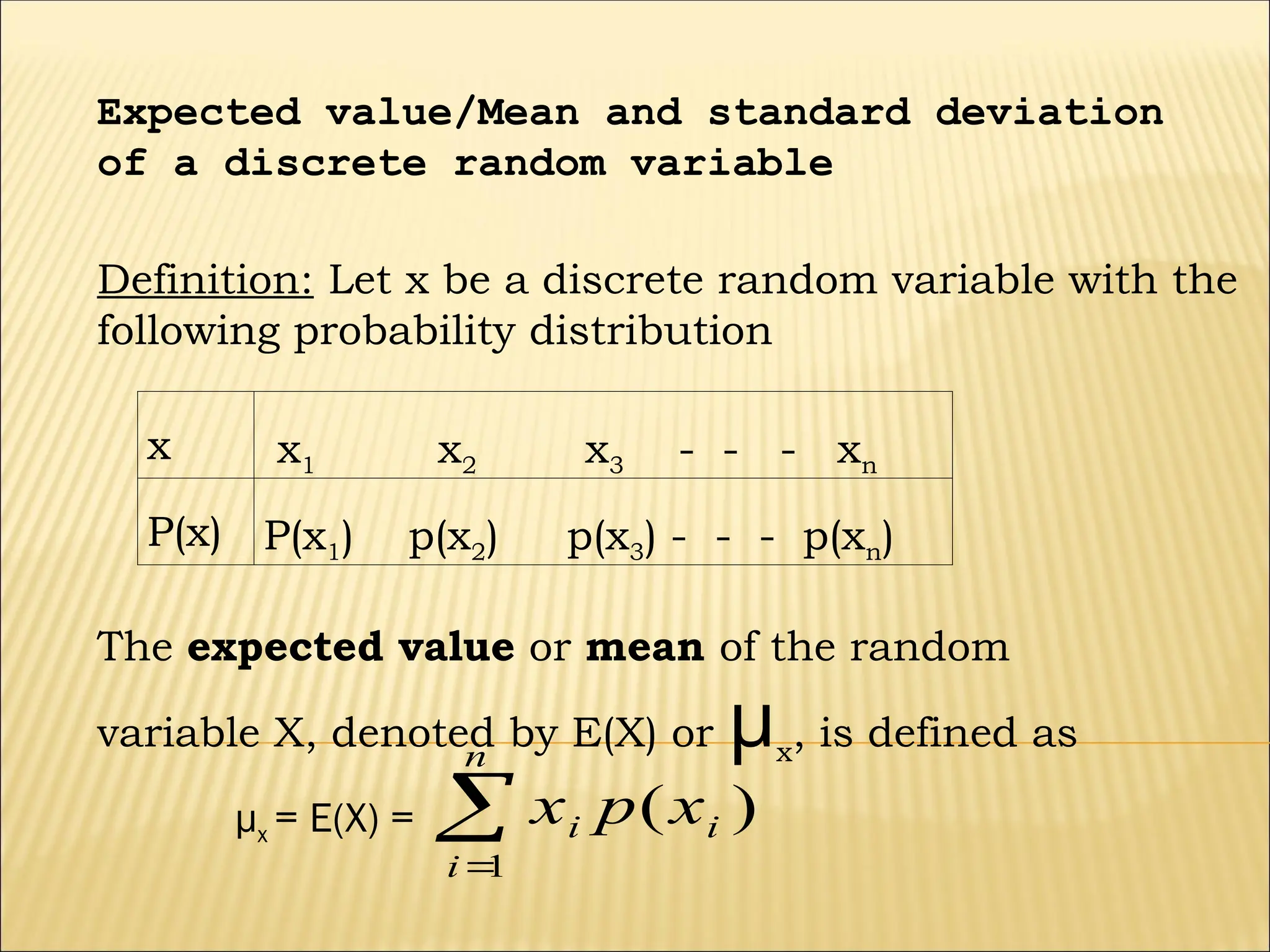
The collection of all pairs [xi
, p(xi
)], i= 1, 2,…
n. is called the probability distribution of the
random variable x.
(i.e. it is a function that associates random
values with their corresponding probabilities.)
This is usually written in the form of a table of x
and p(x)
x x1 x2 x3 - - - xn
P(x) P(x1) p(x2) p(x3)- - -- p(xn )

17. x 0 1 2 3 4
P(x) 1/16 4/16 6/16 4/16 1/16
Example
Toss a coin four times and find the probability
distribution of obtaining heads.
Soln
Let X be number of heads obtained in tossing a coin 4
times; x = 0 1, 2, 3, 4
.
Note that p(x) is a probability function

18. x x1 x2 x3 - - - xn
P(x) P(x1) p(x2) p(x3) - - - p(xn)
Expected value/Mean and standard deviation
of a discrete random variable
Definition: Let x be a discrete random variable with the
following probability distribution
The expected value or mean of the random
variable X, denoted by E(X) or µx
, is defined as
µx = E(X) = 

n
i
i
i x
p
x
1
)
(

19. And the variance of x, denoted by  x
2
or var(X), is given
by
2
x = var(X) =
or,
)
(
)
( 2
1
i
x
n
i
i x
p
x 



Then the standard deviation of x, denoted by Sx or s.d,
is simply the positive square root of the variance
i.e  x 


n
i
i
x
i x
p
x
1
2
)
(
)
( 
= s.d(X)=
2
1
2
2
)
( x
n
i
i
i
x x
x
P 
 



20. x 0 1 2 3
P(x) 1/8 3/8 3/8 1/8
Examples
1.Toss a coin 3 times and find the expected number
of tails obtained and its standard deviation
Solution
Let X = number of tails obtained
X = x, x = 0, 1, 2, 3.

21. The expected number of tail/s obtained is
µx = E(x) = 

3
0
)
(
i
i
i x
p
x
= 0X1/8+1X3/8+2X3/8 + 3X1/8
=12/8
= 3/2
= 1.5 tails
Therefore, 1 tail or 2 tails are equally expected in
tossing a con 3 times

22. 2
x = var(x) = )
(
)
( 2
1
i
x
n
i
i x
p
x 



= (0- 3/2)2
X1/8 +(1-3/2)2
X3/8 +(2-3/2)2
X3/8
+(3.3/2)2
X1/8
= 3/4
The standard deviation or the fluctuation or
uncertainity from the expected value 1.5 tails is
σx = s.d = )
(x
Var
4
/
3
=

= 
3/2 tails

23. 2. A study shows that the following is data of the number of
crises that could occur during the day off for the manager of a
business
No of crises (xi) probabilities (p(xi))
0 0.37
1 0.31
2 0.18
3 0.09
4 0.04
5 0.01
Find the expected number of crises and the standard deviation of
the crises during the day off.

24. Solution
Let x = No of crises during the day off
X = x, x = 0, 1, 2, 3, 4, 5.
= E(x) = 

5
0
)
(
i
i
i x
p
x = 1.15 crises



5
0
2
)
(
)
(
i
i
x
i x
p
x  41
.
1
x = s.d = = = 1.19 crises
Therefore, the expected number of crises during the day
off for the manager is 1.15 crises and the fluctuation
from the mean or expected number of crises is plus or
minus 1.19 crises.
µx

25. NB:
•The concept of probability distribution is the underlying foundation
of most inferential statistical analysis.
•An understanding of probability distributions is critical in using
quantitative methods such as estimation, hypothesis testing,
regression.
•Distribution means shape or form of data.
•There are few standard shapes of data or distributions.
• Among them, binomial, Poisson and normal distributions are the
most common distributions.
•A random variable X could possibly take any one of these basic
distributions

26. Binomial Distribution
•It is an example of discrete probability distribution (it is
applicable only for discrete random variable).
•A binomial random variable represents the number of successes in
a fixed number of independent trials, each with the same
probability of success.
The binomial distribution is a probability distribution that
models the number of successful outcomes in a fixed number of
Bernoulli trials, where each trial has two possible outcomes
(usually denoted as success and failure) and the trials are
independent and have the same probability of success.
•If a random variable is discrete, then the distribution it takes is a
discrete probability distribution.

27. Examples of binomial random variables
Example 1. Customer retention in a subscription model: Suppose a company
runs a marketing campaign to retain its subscription customers. If the
company knows that 60% of its current customers renew their subscriptions
after the campaign, a binomial random variable can represent the number of
customers (successes) who renew their subscriptions out of a fixed number of
100 customers contacted.
Success is defined as a customer renewing the subscription, and each customer has
two possible outcomes: renew (success) or not renew (failure).
Example 2. Email marketing campaign response: A company sends out 500
promotional emails to potential customers, and the historical data shows a
10% success rate in getting a positive response (e.g., a customer clicks on a
link or makes a purchase). Here, the number of positive responses from these
500 emails can be modeled by a binomial distribution.
The two possible outcomes for each email are either a response (success) or no
response (failure).

28. Example 3: Select n students randomly and identify the sex ( male or female
only)
Example 4: Select n items randomly and check for defectiveness (defective or
non- defective)
Example 5: Select n patients randomly in a hospital and check whether or not
they survived (die or survive)
Binomial random variables are commonly used in the field of Marketing
Management to model situations involving binary outcomes or multiple trials
with a fixed probability of success.

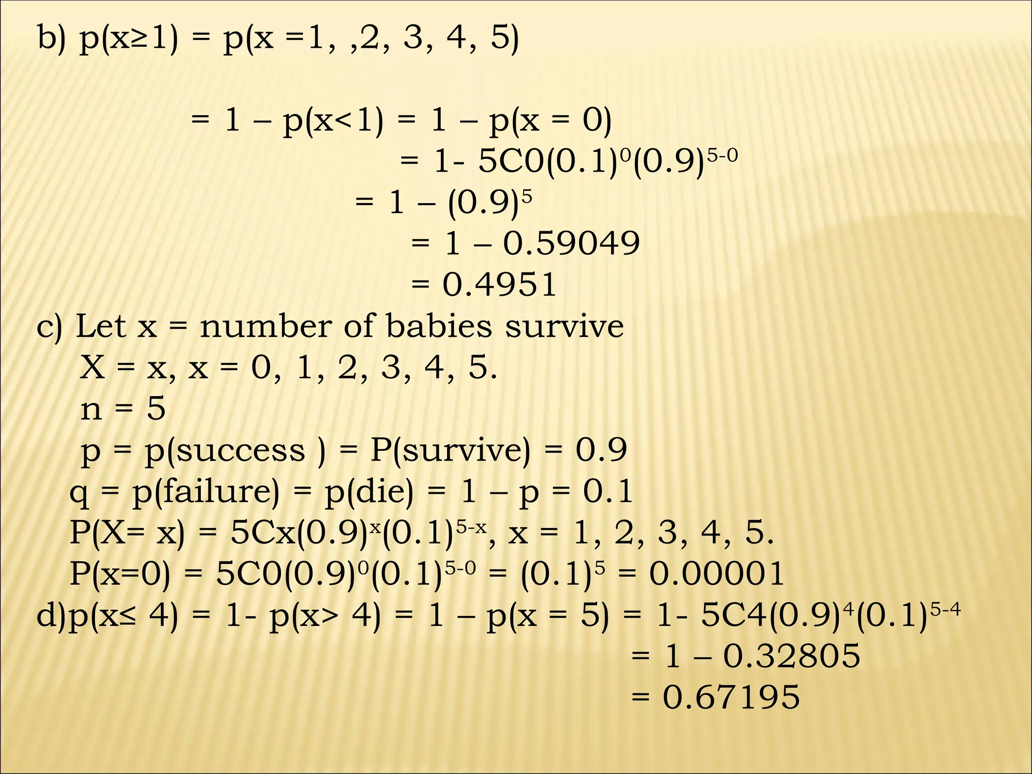
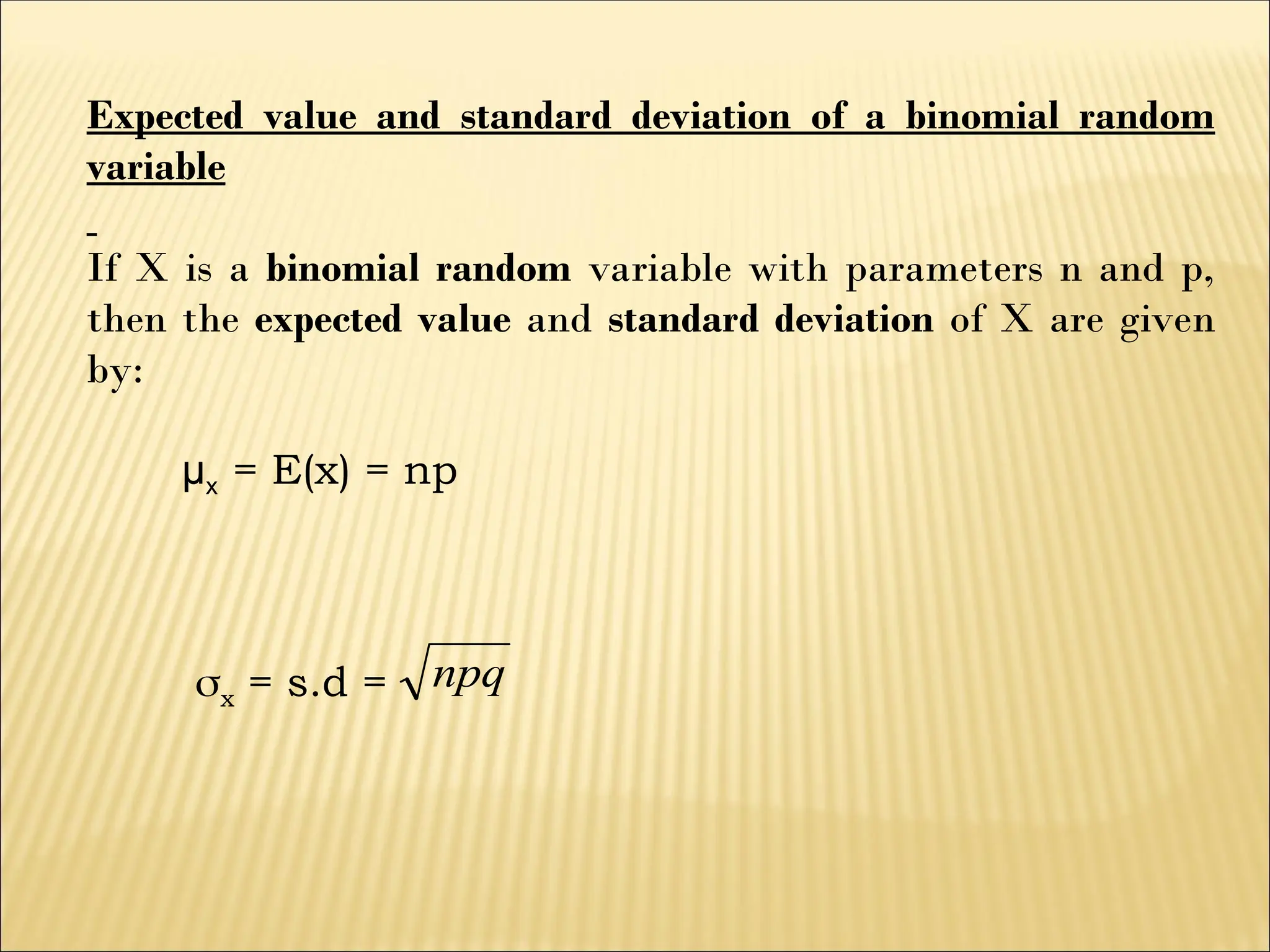
29. Definition: If a random variable X is binomial in n independent trials with
probability (p) of success and probability [(1-p) or q] of failure on a single
trial, then the probability function of the random variable X is called
binomial distribution, which is given by:
P(X = x) = px
qn-x
, x = 0, 1, 2, ---, n.
)
( x
n
)!
(
!
!
x
n
x
n

where, p = p(success),
q = p(failure),
n = number of trials
=
)
( x
n
nCx =

30. NB:
1. A binomial distribution is identified or specified by two parameters n and p.
2. If a random variable X is binomial with parameters n and p, then it is written
as X B(n, p)

31. Examples
1.A study shows that 30% of items produced by a factory are
defective. If a random sample of 4 items are selected, what is
the probability that
a) Exactly 2 of them are defective
b) At most 1 is defective
Exercise:
what is the probability that
i) Not less than 2 are non – defective. Ans: 0.3483
ii) At least 1 is non-defective.
Ans: 0.9919

32. Solution
Let X = number of defective items
n = 4 = number of trials
X = x, x = 0, 1, 2, 3, 4.
Outcomes at each trial are, defective or non-
defective.
Therefore, X is a binomial random variable.
i. e. X B(n, p)
n = 4
p = p(success) = p( defective) = 30% = 0.3
q = p( failure) = p( non – defective)=1- p = 0.7

33. p(X = x) = 4Cx(0.3)x
(0.7)4-x
, x = 0, 1, 2, 3, 4.
a) p(X =2) = 4C2(0.3)2
(0.7)4-2
= 6X0.09X0.49 = 0.2646
b) p(X ≤ 1) = p(X = 0,1) = P(X =0) + p(X=1)
= 4C0(0.3)0
(0.7)4-0
+4C1(0.3)1
(0.7)4-1
= 0.2401+0.4116
= 0.6517

34. Example 2. Medical sources show that one in ten babies
admitted to a hospital die of certain disease. Suppose that a
random sample of five babies are selected from hospitals, what
is the probability that
a) More than 2 babies die
b) at least 1 baby die
c) no baby survives
d) at most 4 babies survive

35. Solution
Let X = number of babies die
n = 5 – number of trials
X = x, x = 0, 1, 2, 3, 4, 5.
Outcomes at each trial are exactly two, die or survive
 X  B(n,p)
n= 5, p= p(success) = p( die) = 0.1
q = p(failure) = 1 – p = 0.9
p(X=x) = 5Cx(0.1)x
(0.9)5-x
, x =0, 1, 2, 3, 4, 5
a) p(X > 2) = p(X = 3,4,5)
= 5C3(0.1)3
(0.9)5-3
+5C4(0.1)4
(0.9)5-4
+ 5C5(0.1)5
(0.9)5-5
= 0.0081+0.00045+0.00001
= 0. 00856

36. b) p(x≥1) = p(x =1, ,2, 3, 4, 5)
= 1 – p(x<1) = 1 – p(x = 0)
= 1- 5C0(0.1)0
(0.9)5-0
= 1 – (0.9)5
= 1 – 0.59049
= 0.4951
c) Let x = number of babies survive
X = x, x = 0, 1, 2, 3, 4, 5.
n = 5
p = p(success ) = P(survive) = 0.9
q = p(failure) = p(die) = 1 – p = 0.1
P(X= x) = 5Cx(0.9)x
(0.1)5-x
, x = 1, 2, 3, 4, 5.
P(x=0) = 5C0(0.9)0
(0.1)5-0
= (0.1)5
= 0.00001
d)p(x≤ 4) = 1- p(x> 4) = 1 – p(x = 5) = 1- 5C4(0.9)4
(0.1)5-4
= 1 – 0.32805
= 0.67195

37. Exercises
1. A company produces electronic components, and on average,
5% of the components are defective. A quality control team
randomly selects 10 components for inspection. What is the
probability that exactly 2 of the components are defective?
2. A bank receives loan applications, and historically, 80% of
the applications are approved. If the bank receives 20 loan
applications, what is the probability that at most 2 applications
are approved?

38. Expected value and standard deviation of a binomial random
variable
If X is a binomial random variable with parameters n and p,
then the expected value and standard deviation of X are given
by:
µx = E(x) = np
x = s.d = npq

39. Poisson distribution
•Poisson distribution: is an example of discrete probability
distribution.
•It models the number of events that occur within a fixed
interval of time or space.
A Poisson random variable represents the number of events
occurring in a fixed interval of time or space.
Examples of Poisson random variable:
1. Let X be number of accidents in one year
X= x, x= 0, 1, 2, ---
 x accidents/year
Event- accident
Unit – year

40. Examples of Poisson random variables
Example 1. Number of customer complaints per day: A customer service
department of a company might receive an average of 3 complaints per day.
The number of complaints received per day can be modeled by a Poisson
random variable, as complaints happen randomly and independently over
time.
Example 2. Foot traffic in a retail store: Imagine a marketing manager of a
retail store tracks the number of customers entering the store in an hour. If
historical data suggests that the store gets an average of 20 customers per
hour, the number of customers arriving in any given hour could follow a
Poisson distribution. This would help the store adjust staffing or
promotional efforts based on expected customer flow.

41. Example 3. Let X is be number of errors per page
X= x, x= 0, 1, 2, ---
 x errors/page
Event – error
Unit – page
Example 4. Let X be number of customers arriving at a bank
in one minute
X= x, x= 0, 1, 2, ---
 x customers/minute
Event – arrival of customers
Unit – minute
Etc…

42. Let  be average number of events per unit. Then T = average number of
events occurring in T units.
•If X is the average number of events in T units, then X is a random
variable that satisfies Poisson law, which is called the Poisson distribution,
and is given by
!
)
(
x
T
e x
T



, x = 0, 1, 2, ----
P (X = x) =
where, e = 2. 71826 (irrational numbers)

43. If T = 1, then, P (X = x) =
!
)
(
x
e x



=, x = 0, 1, 2, ---
Note:
The Poisson distribution is specified by a single parameter, , and
is written as, X P().

44. Example 2: Suppose a company experiences an average of 4
transaction errors per day in its financial records. What is the
probability of observing exactly 2 errors in a given day? In 2
days’ time?
Answer: 0.14653; 0.01073
Example 3: Suppose that on a given hour the number of ships
arriving at a port has mean 2.3. What is the probability that there
will be
a) Exactly 3 ships arriving at the port in 2 hrs.
b) At most one ship arrives at the port in one hr.
c) At least 2 ships arrive at the port in 30 minutes.
Example 1: The average number of customers entering a retail
store in one hour is 20. What is the probability that exactly 25
customers will enter the store in the next 2 hours? Answer: 0.0031

45. Example 3: Solution
Let X = number of ships arriving at a port in one hr
X=x, x = 0, 1, 2, ---
 = Average number of ships arriving at a port/hr
= 2.3 ships/hr
 X is a Poisson random variable i.e X P()
P (X = x) =
!
)
(
x
T
e x
T



, x = 0, 1, 2, ----

46. a)  = 2.3
T = 2  T = 2.3x2 = 4.6
!
)
(
x
T
e x
T



6
)
6
.
4
(
0101
.
0 3
P(X = 3) =
6
)
6
.
4
( 3
6
.
4

e
=
=
= 0.164

47. b)  = 2.3
T = 1  T = 2.3
P(X≤ 1) = p(X = 0,1) =
1
)
3
.
2
( 0
3
.
2

e +
1
)
3
.
2
( 1
3
.
2

e
= 3.3e-2.3
= 3.3X0.1003
= 0.33099

48. c)  = 2.3
T = 0.5  T = 2.3x0.5 = 1.15
P(X≥ 2) = 1 – p(x < 2) = 1 – p(X =0,1)
1 -
1
)
15
.
1
( 0
15
.
1

e
=
= 1- e-1.15
(1 + 1.15)
= 1 – 0.317X2.15
= 0.31845
-
1
)
15
.
1
( 1
15
.
1

e
-

49. Exercise
1.A retail store receives an average of 10 customers per hour during its peak
hours. What is the probability of having at most 5 customers in the next hour?
2.A manufacturing facility experiences an average of 2 equipment failures per
week. What is the probability of having more than 3 failures in 4 weeks’ time?
3.The average number of customer support calls a service desk receives in 30
minutes is 10. What is the probability that fewer than 5 calls will be received in
the next 30 minutes?
4. The average number of network packets arriving at a server in one second is
15. What is the probability that the server will receive no more than 10
packets in the next second?
5. The average number of visits to a website per minute is 8. What is the
probability of having exactly 12 visits in the next minute?

50. Note
If X be a Poisson random variable with parameter , then the
expected value and standard deviation of X can be shown to be
µx
= E(x) = 
2
x = var(x) = 
x = s.d = 

51. Poisson approximation to binomial (Assignment)

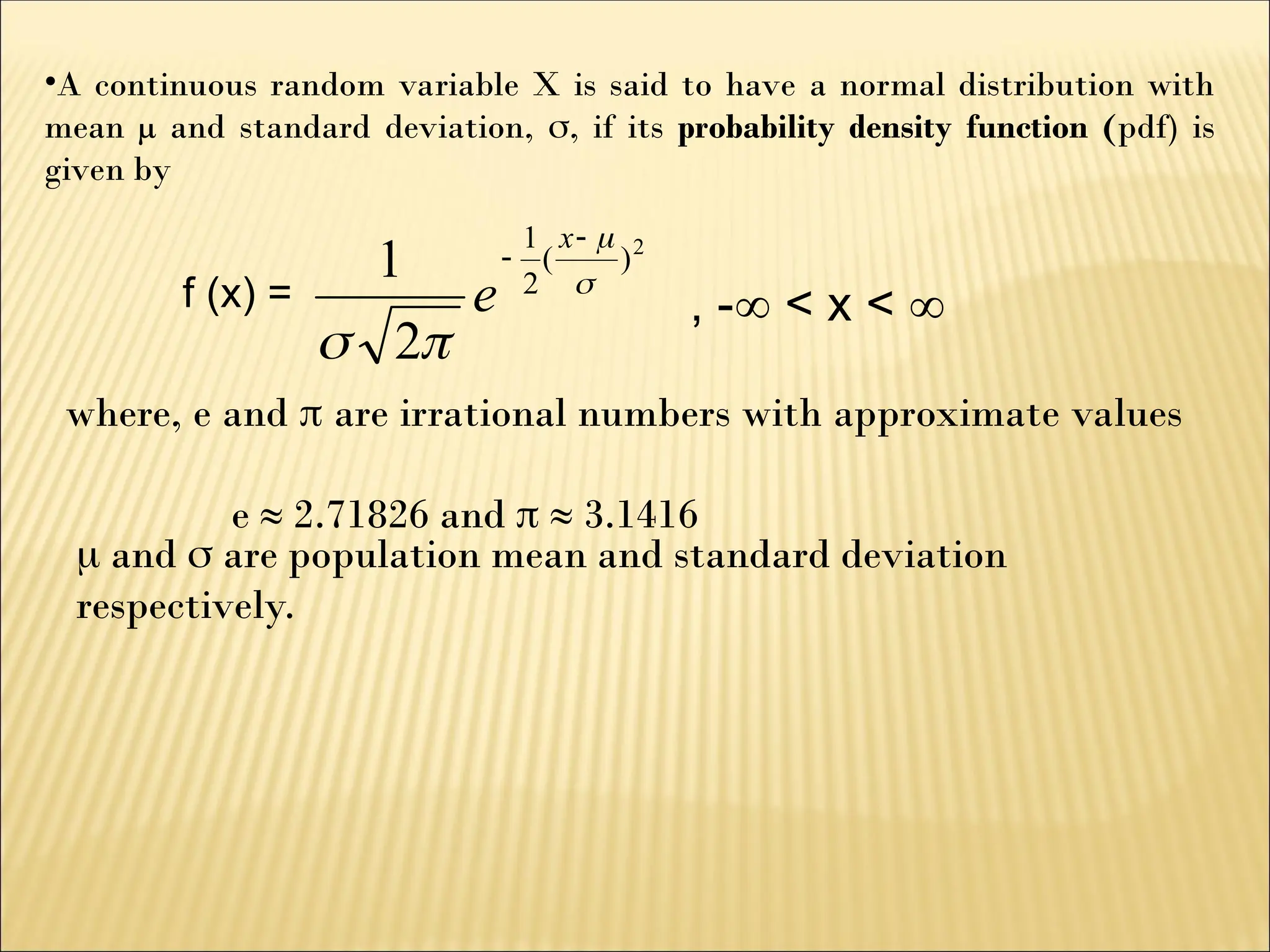
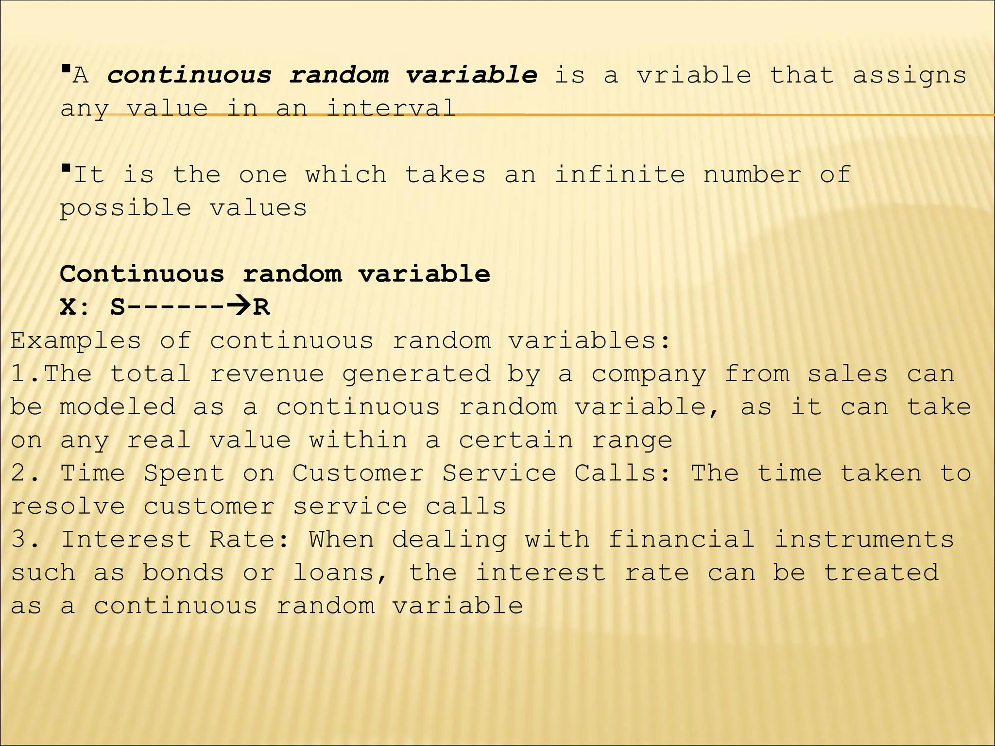
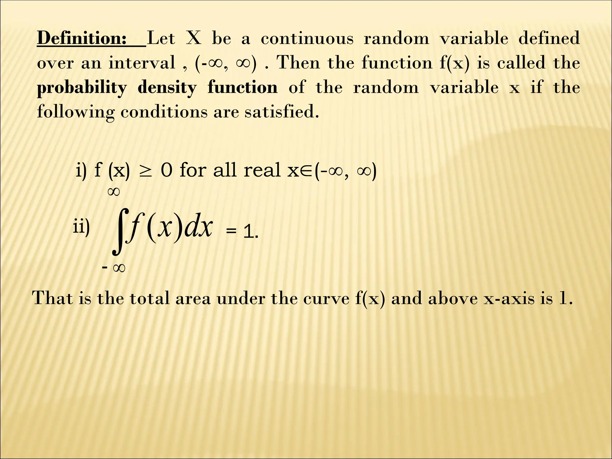
52. Continuous probability distributions
A continuous probability distribution is one in which a continuous
random variable X can take on any value within a given range of
values which can be infinite, and therefore uncountable.
‒
A continuous random variable X is represented by an interval,
a ≤ X≤ b or [a, b] – having infinitely many values.
And the probability function is also represented by the continuous
function, f(x), which is called probability density function (pdf).

53. Definition: Let X be a continuous random variable defined
over an interval , (-, ) . Then the function f(x) is called the
probability density function of the random variable x if the
following conditions are satisfied.
i) f (x)  0 for all real x(-, )




dx
x
f )
( = 1.
ii)
That is the total area under the curve f(x) and above x-axis is 1.

54. NB:
Let f(x) be a probability density function of a continuous random
variable X defined over an interval [a, b]. Then
a)The probability that x lies in the interval [c, d] is
given by
P(c  x  d) =

d
c
dx
x
f )
(

55. b) The expected value and standard deviation of X is also be given as
 = E (x) =

b
a
dx
x
xf )
(
And the variance of x is
V (x) = 2
=  
b
a
dx
x
f
x )
(
)
( 2

Therefore, the standard deviation of x is
 =
)
(x
v

56. Normal distribution
•It is an example of a continuous probability distribution.
•Normal distribution is a continuous probability distribution that is symmetrical around
its mean, most of the observations cluster around the central peak, and the probabilities
for values further away from the mean taper off equally in both directions.
•The normal distribution, also known as the Gaussian distribution, has numerous
practical applications in Marketing Management.

57. •A continuous random variable X is said to have a normal distribution with
mean µ and standard deviation, , if its probability density function (pdf) is
given by
f (x) =
2
)
(
2
1
2
1 





x
e , - < x < 
where, e and  are irrational numbers with approximate values
e ≈ 2.71826 and  ≈ 3.1416
 and  are population mean and standard deviation
respectively.

58. Normal distribution is specified by two parameters µ and
The graph of the normal distribution, f(x), is the familiar bell-
shaped curve called normal curve
f(x),
y
x
µ
, and is written as
X  N( µ, 2
)

59. The normal curve has the following properties.
It is bell-shaped curve
It is symmetrical about its mean.
The total area below f(x) and above the x- axis is 1
 The area to the right of  = area to left of  = 3. It is
asymptotic to the x-axis.
The mean, median and mode are almost identical
 It is asymptotic to the x-axis.

60. Definition. A normal distribution with mean zero and standard
deviation one is known as the standard normal distribution or
Z – distribution with the resulting pdf
f (z) =
2
2
1
2
1 z
e


, -  < x < 

61. NB:
1, Any continuous random variable X  N(, 2
) can be
standardized using the transformation
Z =



x
i. e, if X  N(, 2
), then Z  N(0, 1)
2. A normal table is a standard normal table.

62. How to read from normal table
After standardization, reading from normal table is possible if it
is in the form
p(0 < Z < a)
where, a = a positive number less than or equal to 3.09
i.e, p(0 < Z < a) = the area under the normal curve
between o and a
f (z)
P (0< Z < a)
a
0

63. above readable form to use the standard normal table
Examples
- P(0<Z<2.34) = 0.4904
-P(- 1.63< Z < 0)= p(0<Z<1.63)= 0.4484 – since
the curve is symmetric
-P(Z<1.05) = 0.5 + p(0<Z<1.05) = 0.5 + 0.3531
= 0.8532
-P(Z< -2.35) = 0.5 – p(0<Z<2.35) =0.5 – 0.4906
= 0.0094
-P(-1.43<Z<2.11)= p(0<Z<1.43) +p(0<Z<2.11)
= 0.4236 +0.4826= 0.9062
-P(-2.34<Z<-1.03) = p(0<Z<2.34) – p(0<Z<1.03)
= 0.4904 -0.3485= 0.1419
Etc

64. Example
The age of workers of an industry is normally distributed with
mean 35 years and standard deviation of 5 years.
i)What is the probability that a randomly selected
worker is
a) Less than 40 years of age
b) Between 28 and 37 years of age
c) at least 42 years of age
ii) Find the age
a)Below which 80% of workers have it
b) Above which 60% of workers have it

65. Solution
Let X = the age of the selected worker
X = x, 18 ≤ X ≤ 60 – continuous random variable.
But X  N(, 2
) – given
i) a) p(X < 40) = p )
5
35
40
(





x
= P(Z < 1)
= 0.5 +p(0<Z<1)
= 0.5 + 0.3413
= 0.8413
p(28<X<37)= p( )
5
35
37
5
35
28 






x
= p(-1.4<Z<0.4)
= p(0<Z<1.4) +p(<Z<0.4)
= 0.4192 + 0.1554 = 0.5746

66. c) p(X≥ 42) = p( )
5
35
42
(





x
= p(Z≥1.4)= 0.5 – p(0<Z<1.4)
= 0.5 – 0.4192 = 0.0808
ii) a) Let xo = the age below which 80% of workers
have it
0.5
0.3
0.2
= 35 x0

67. 0.5 0.3
0.2
= 0
5
35
0 
x
 p(0 < Z <
5
35
0 
x ) = 0.3

5
35
0 
x = 0.84
 xo
= 35 +0.84X5 = 39.2 years

68. b)Let xo
= the age above which 60% of
workers have it
0.4
0.1
0.5
xo = 35
-
)
5
35
0
(


x
= 0
0.4
0.1 0.5

69. p(-( )< Z < 0) = 0.1
 -(
5
35
0 
x
) = 0.25

5
35
0 
x
= - 0.25
5
35
0 
x
 xo = 35 – 0.25X 5 = 33.75 years

70. Exercises
1. The salary of workers of an industry is normally distributed with mean
salary of $420 and standard deviation of $55. If any one worker from the
industry is selected randomly,
i) What is the probability that he or she has salary of
a) More than $450 b) Less than $300 c) Between $380 and $490
ii) What is the salary
a) Below which 5% of workers have it
b) Above which 35% of workers have it
2.The average monthly expense on office supplies for a company is $5,000,
with a standard deviation of $800. Assuming the expense follows a normal
distribution, what is the probability that the company's monthly office supply
expense will be between $4,200 and $5,800?
3.An investment firm is analyzing the monthly returns of a certain stock. The
returns follow a normal distribution with a mean of 1.5% and a standard
deviation of 2.2%. What is the probability that the stock will have a negative
return in the next month?

71. Normal approximation to binomial (Assignment)
4.An auditing firm is investigating the distribution of purchase amounts in a
dataset to identify potential fraudulent transactions. The purchase amounts
are normally distributed with a mean of $500 and a standard deviation of
$100. What percentage of transactions have purchase amounts exceeding
$700?

72. THE END OF CHAPTER ONE