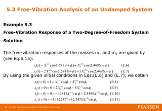
This document chapter discusses two-degree-of-freedom vibrational systems. It introduces two-degree-of-freedom models and defines generalized coordinates. It derives the equations of motion for forced vibration of a damped two-mass spring system. It then analyzes the free vibration of an undamped two-degree system, determining the natural frequencies from the characteristic equation. The normal modes of vibration are expressed in terms of the natural frequencies and mode shapes.

2. Mechanical Vibrations
Fifth Edition in SI Units
Singiresu S. Rao

3. © 2011 Mechanical Vibrations Fifth Edition in SI Units
3
Chapter 5
Two Degree Freedom Systems

4. © 2011 Mechanical Vibrations Fifth Edition in SI Units
4
Chapter Outline
5.1 Introduction
5.2 Equations of Motion for Forced Vibration
5.3 Free Vibration Analysis of an Undamped System
5.4 Torsional System
5.5 Coordinate Coupling and Principal Coordinates
5.6 Forced-Vibration Analysis
5.7 Semidefinite Systems
5.8 Self-Excitation and Stability Analysis
5.9 Transfer-Function Approach
5.10 Solutions Using Laplace Transform
5.11 Solutions Using Frequency Transfer Functions

5. © 2011 Mechanical Vibrations Fifth Edition in SI Units
5
5.1
Introduction

6. © 2011 Mechanical Vibrations Fifth Edition in SI Units
6
5.1 Introduction
• Two-degree-of-freedom systems are defined as systems that
require two independent coordinates to describe their motion.
• For simplicity, a two-degree-of-freedom model can be used as
shown in the figure.

7. © 2011 Mechanical Vibrations Fifth Edition in SI Units
7
5.1 Introduction
• The general rule for the computation of the number of degrees of
freedom can be stated as follows:
=
No. of degrees
of freedom of
the system
No. of masses in the
system x no. of
possible types of
motion of each mass

8. © 2011 Mechanical Vibrations Fifth Edition in SI Units
8
5.1 Introduction
• As is evident from the systems shown in figures earlier on, the
configuration of a system can be specified by a set of independent
coordinates termed as generalized coordinates, such as length,
angle, or some other physical parameters.
• Principle coordinates is defined as any set of coordinates that leads
a coupled equation of motion to an uncoupled system of equations.

9. © 2011 Mechanical Vibrations Fifth Edition in SI Units
9
5.2
Equations of Motion for Forced Vibration

10. © 2011 Mechanical Vibrations Fifth Edition in SI Units
10
5.2 Equations of Motion for Forced Vibration
• Consider a viscously damped two-degree-of-freedom spring-mass
system, shown in the figure below

11. © 2011 Mechanical Vibrations Fifth Edition in SI Units
11
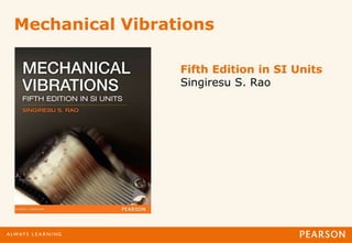
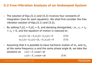
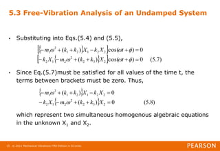
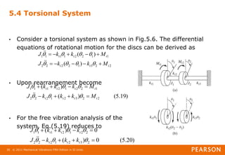
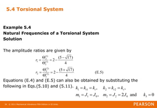
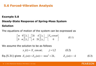
5.2 Equations of Motion for Forced Vibration
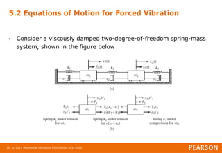
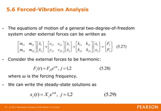
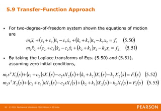
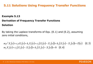
• The application of Newton’s second law of motion to each of the
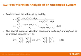
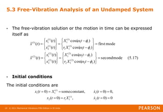
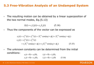
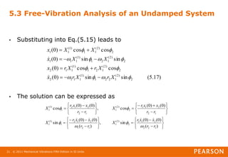
masses gives the equations of motion:
• Both equations can be written in matrix form as
where [m], [c], and [k] are called the mass, damping, and stiffness
matrices, respectively, and are given by
)
2
.
5
(
)
(
)
(
)
1
.
5
(
)
(
)
(
2
2
3
2
1
2
2
3
2
1
2
2
2
1
2
2
1
2
1
2
2
1
2
1
1
1
F
x
k
k
x
k
x
c
c
x
c
x
m
F
x
k
x
k
k
x
c
x
c
c
x
m






















)
3
.
5
(
)
(
)
(
]
[
)
(
]
[
)
(
]
[ t
F
t
x
k
t
x
c
t
x
m











12. © 2011 Mechanical Vibrations Fifth Edition in SI Units
12
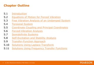
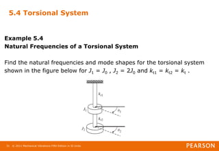
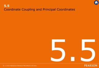
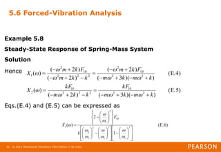
5.2 Equations of Motion for Forced Vibration
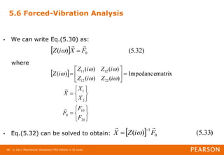
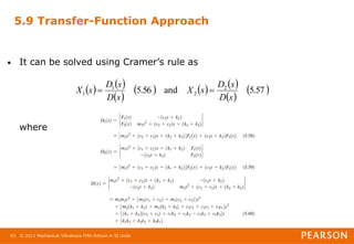
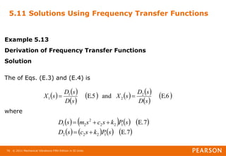
• We have
• And the displacement and force vectors are given respectively:
• It can be seen that the matrices [m], [c], and [k] are symmetric:
where the superscript T denotes the transpose of the matrix.





























3
2
2
2
2
1
3
2
2
2
2
1
2
1
]
[
]
[
0
0
]
[
k
k
k
k
k
k
k
c
c
c
c
c
c
c
m
m
m














)
(
)
(
)
(
)
(
)
(
)
(
2
1
2
1
t
F
t
F
t
F
t
x
t
x
t
x


]
[
]
[
],
[
]
[
],
[
]
[ k
k
c
c
m
m T
T
T




13. © 2011 Mechanical Vibrations Fifth Edition in SI Units
13
5.3
Free-Vibration Analysis of an Undamped System

14. © 2011 Mechanical Vibrations Fifth Edition in SI Units
14
5.3 Free-Vibration Analysis of an Undamped System
• The solution of Eqs.(5.1) and (5.2) involves four constants of
integration (two for each equation). We shall first consider the free
vibration solution of Eqs.(5.1) and (5.2).
• By setting F1(t) = F2(t) = 0, and damping disregarded, i.e., c1 = c2
= c3 = 0, and the equation of motion is reduced to:
• Assuming that it is possible to have harmonic motion of m1 and m2
at the same frequency ω and the same phase angle Φ, we take the
solutions as
)
5
.
5
(
0
)
(
)
(
)
(
)
(
)
4
.
5
(
0
)
(
)
(
)
(
)
(
2
3
2
1
2
2
2
2
2
1
2
1
1
1








t
x
k
k
t
x
k
t
x
m
t
x
k
t
x
k
k
t
x
m




)
6
.
5
(
)
cos(
)
(
)
cos(
)
(
2
2
1
1








t
X
t
x
t
X
t
x

15. © 2011 Mechanical Vibrations Fifth Edition in SI Units
15
5.3 Free-Vibration Analysis of an Undamped System
• Substituting into Eqs.(5.4) and (5.5),
• Since Eq.(5.7)must be satisfied for all values of the time t, the
terms between brackets must be zero. Thus,
which represent two simultaneous homogenous algebraic equations
in the unknown X1 and X2.
 
 
 
  )
7
.
5
(
0
)
cos(
)
(
0
)
cos(
)
(
2
3
2
2
2
1
2
2
2
1
2
1
2
1


















t
X
k
k
m
X
k
t
X
k
X
k
k
m
 
  )
8
.
5
(
0
)
(
0
)
(
2
3
2
2
2
1
2
2
2
1
2
1
2
1










X
k
k
m
X
k
X
k
X
k
k
m



16. © 2011 Mechanical Vibrations Fifth Edition in SI Units
16
5.3 Free-Vibration Analysis of an Undamped System
• For trivial solution, i.e., X1 = X2 = 0, there is no solution. For a
nontrivial solution, the determinant of the coefficients of X1 and X2
must be zero:
which is called the frequency or characteristic equation.
 
 
0
)
(
)
(
det
2
1
2
1
2
2
2
1
2
1
















k
k
m
k
k
k
k
m


 
  )
9
.
5
(
0
)
)(
(
)
(
)
(
)
(
2
2
3
2
2
1
1
3
2
2
2
1
4
2
1









k
k
k
k
k
m
k
k
m
k
k
m
m 


17. © 2011 Mechanical Vibrations Fifth Edition in SI Units
17
5.3 Free-Vibration Analysis of an Undamped System
• Hence the roots are:
• The roots are called natural frequencies of the system.
)
10
.
5
(
)
)(
(
4
)
(
)
(
2
1
)
(
)
(
2
1
,
2
/
1
2
1
2
2
3
2
2
1
2
2
1
1
3
2
2
2
1
2
1
1
3
2
2
2
1
2
2
2
1





 












 







 



m
m
k
k
k
k
k
m
m
m
k
k
m
k
k
m
m
m
k
k
m
k
k




18. © 2011 Mechanical Vibrations Fifth Edition in SI Units
18
5.3 Free-Vibration Analysis of an Undamped System
• To determine the values of X1 and X2,
• The normal modes of vibration corresponding to ω1
2 and ω2
2 can be
expressed, respectively, as
)
11
.
5
(
)
(
)
(
)
(
)
(
3
2
2
2
2
2
2
2
1
2
2
1
)
2
(
1
)
2
(
2
2
3
2
2
1
2
2
2
2
1
2
1
1
)
1
(
1
)
1
(
2
1
k
k
m
k
k
k
k
m
X
X
r
k
k
m
k
k
k
k
m
X
X
r






















)
12
.
5
(
and )
2
(
1
2
)
2
(
1
)
2
(
2
)
2
(
1
)
2
(
)
1
(
1
1
)
1
(
1
)
1
(
2
)
1
(
1
)
1
(












































X
r
X
X
X
X
X
r
X
X
X
X



19. © 2011 Mechanical Vibrations Fifth Edition in SI Units
19
5.3 Free-Vibration Analysis of an Undamped System
• The free-vibration solution or the motion in time can be expressed
itself as
• Initial conditions
The initial conditions are
(5.17)
mode
second
)
cos(
)
cos(
)
(
)
(
)
(
mode
first
)
cos(
)
cos(
)
(
)
(
)
(
2
2
)
2
(
1
2
2
2
)
2
(
1
)
2
(
2
)
2
(
1
)
2
(
1
1
)
1
(
1
1
1
1
)
1
(
1
)
1
(
2
)
1
(
1
)
1
(


























































t
X
r
t
X
t
x
t
x
t
x
t
X
r
t
X
t
x
t
x
t
x


0
)
0
(
,
)
0
(
,
0
)
0
(
constant,
some
)
0
(
2
)
(
1
2
1
)
(
1
1









t
x
X
r
t
x
t
x
X
t
x
i
i
i



20. © 2011 Mechanical Vibrations Fifth Edition in SI Units
20
5.3 Free-Vibration Analysis of an Undamped System
• The resulting motion can be obtained by a linear superposition of
the two normal modes, Eq.(5.13)
• Thus the components of the vector can be expressed as
• The unknown constants can be determined from the initial
conditions:
)
14
.
5
(
)
(
)
(
)
( 2
2
1
1 t
x
c
t
x
c
t
x





)
15
.
5
(
)
cos(
)
cos(
)
(
)
(
)
(
)
cos(
)
cos(
)
(
)
(
)
(
2
2
)
2
(
1
2
1
1
)
1
(
1
1
)
2
(
2
)
1
(
2
2
2
2
)
2
(
1
1
1
)
1
(
1
)
2
(
1
)
1
(
1
1




















t
X
r
t
X
r
t
x
t
x
t
x
t
X
t
X
t
x
t
x
t
x
)
16
.
5
(
)
0
(
)
0
(
),
0
(
)
0
(
),
0
(
)
0
(
),
0
(
)
0
(
2
2
2
2
1
1
1
1
x
t
x
x
t
x
x
t
x
x
t
x













21. © 2011 Mechanical Vibrations Fifth Edition in SI Units
21
5.3 Free-Vibration Analysis of an Undamped System
• Substituting into Eq.(5.15) leads to
• The solution can be expressed as
)
17
.
5
(
sin
sin
)
0
(
cos
cos
)
0
(
sin
sin
)
0
(
cos
cos
)
0
(
2
)
2
(
1
2
2
1
)
1
(
1
1
1
2
2
)
2
(
1
2
1
)
1
(
1
1
2
2
)
2
(
1
2
1
)
1
(
1
1
1
2
)
2
(
1
1
)
1
(
1
1












X
r
X
r
x
X
r
X
r
x
X
X
x
X
X
x


















































)
(
)
0
(
)
0
(
sin
,
)
(
)
0
(
)
0
(
sin
)
0
(
)
0
(
cos
,
)
0
(
)
0
(
cos
1
2
2
2
1
1
2
)
2
(
1
1
2
1
2
1
2
1
)
1
(
1
1
2
2
1
1
2
)
2
(
1
1
2
2
1
2
1
)
1
(
1
r
r
x
x
r
X
r
r
x
x
r
X
r
r
x
x
r
X
r
r
x
x
r
X











22. © 2011 Mechanical Vibrations Fifth Edition in SI Units
22
5.3 Free-Vibration Analysis of an Undamped System
• We can obtain the desired solution as
 
   
   
 
   
   
)
18
.
5
(
)
0
(
)
0
(
[
)
0
(
)
0
(
tan
cos
sin
tan
)
0
(
)
0
(
[
)
0
(
)
0
(
tan
cos
sin
tan
)
0
(
)
0
(
)
0
(
)
0
(
)
(
1
sin
cos
)
0
(
)
0
(
)
0
(
)
0
(
)
(
1
sin
cos
2
1
1
2
2
1
1
1
2
)
2
(
1
2
)
2
(
1
1
2
2
1
2
1
2
1
2
1
1
)
1
(
1
1
)
1
(
1
1
1
2
/
1
2
2
2
2
1
1
2
2
1
1
1
2
2
/
1
2
2
)
2
(
1
2
2
)
2
(
1
)
2
(
1
2
/
1
2
1
2
2
1
2
2
2
1
2
1
2
2
/
1
2
1
)
1
(
1
2
1
)
1
(
1
)
1
(
1







































 












 











x
x
r
x
x
r
X
X
x
x
r
x
x
r
X
X
x
x
r
x
x
r
r
r
X
X
X
x
x
r
x
x
r
r
r
X
X
X























23. © 2011 Mechanical Vibrations Fifth Edition in SI Units
23
5.3 Free-Vibration Analysis of an Undamped System
Example 5.3
Free-Vibration Response of a Two-Degree-of-Freedom System
Find the free-vibration response of the system shown in Fig.5.3(a)
with k1 = 30, k2 = 5, k3 = 0, m1 = 10, m2 = 1 and c1 = c2 = c3 = 0 for
the initial conditions .

24. © 2011 Mechanical Vibrations Fifth Edition in SI Units
24
5.3 Free-Vibration Analysis of an Undamped System
Example 5.3
Free-Vibration Response of a Two Degree of Freedom System
Solution
For the given data, the eigenvalue problem, Eq.(5.8), becomes
By setting the determinant of the coefficient matrix in Eq.(E.1) to zero,
we obtain the frequency equation,
(E.1)
0
0
5
5
-
5
35
10
0
0
2
1
2
2
2
1
3
2
2
2
2
2
2
1
2
1























































X
X
X
X
k
k
m
k
k
k
k
m




(E.2)
0
150
85
10 2
4


 


25. © 2011 Mechanical Vibrations Fifth Edition in SI Units
25
5.3 Free-Vibration Analysis of an Undamped System
Example 5.3
Free-Vibration Response of a Two-Degree-of-Freedom System
Solution
The natural frequencies can be found as
The normal modes (or eigenvectors) are given by
E.3)
(
4495
.
2
,
5811
.
1
0
.
6
,
5
.
2
2
1
2
2
2
1








E.5)
(
5
1
E.4)
(
2
1
)
2
(
1
)
2
(
2
)
2
(
1
)
2
(
)
1
(
1
)
1
(
2
)
1
(
1
)
1
(
X
X
X
X
X
X
X
X








































26. © 2011 Mechanical Vibrations Fifth Edition in SI Units
26
5.3 Free-Vibration Analysis of an Undamped System
Example 5.3
Free-Vibration Response of a Two-Degree-of-Freedom System
Solution
The free-vibration responses of the masses m1 and m2 are given by
(see Eq.5.15):
By using the given initial conditions in Eqs.(E.6) and (E.7), we obtain
(E.7)
)
4495
.
2
cos(
5
)
5811
.
1
cos(
2
)
(
(E.6)
)
4495
.
2
cos(
)
5811
.
1
cos(
)
(
2
)
2
(
1
1
)
1
(
1
2
2
)
2
(
1
1
)
1
(
1
1












t
X
t
X
t
x
t
X
t
X
t
x
(E.11)
sin
2475
.
12
1622
.
3
)
0
(
(E.10)
sin
4495
.
2
sin
5811
.
1
0
)
0
(
(E.9)
cos
5
cos
2
0
)
0
(
(E.8)
cos
cos
1
)
0
(
2
)
2
(
1
)
1
(
1
2
2
)
2
(
1
1
)
1
(
1
1
2
)
2
(
1
1
)
1
(
1
2
2
)
2
(
1
1
)
1
(
1
1







X
X
t
x
X
X
t
x
X
X
t
x
X
X
t
x




















27. © 2011 Mechanical Vibrations Fifth Edition in SI Units
27
5.3 Free-Vibration Analysis of an Undamped System
Example 5.3
Free-Vibration Response of a Two-Degree-of-Freedom System
Solution
The solution of Eqs.(E.8) and (E.9) yields
The solution of Eqs.(E.10) and (E.11) leads to
Equations (E.12) and (E.13) gives
(E.12)
7
2
cos
;
7
5
cos 2
)
2
(
1
1
)
1
(
1 
 
 X
X
(E.13)
0
sin
,
0
sin 2
)
2
(
1
1
)
1
(
1 
 
 X
X
(E.14)
0
,
0
,
7
2
,
7
5
2
1
)
2
(
1
)
1
(
1 


 

X
X

28. © 2011 Mechanical Vibrations Fifth Edition in SI Units
28
5.3 Free-Vibration Analysis of an Undamped System
Example 5.3
Free-Vibration Response of a Two-Degree-of-Freedom System
Solution
Thus the free vibration responses of m1 and m2 are given by
(E.16)
4495
.
2
cos
7
10
5811
.
1
cos
7
10
)
(
(E.15)
4495
.
2
cos
7
2
5811
.
1
cos
7
5
)
(
2
1
t
t
t
x
t
t
t
x





29. © 2011 Mechanical Vibrations Fifth Edition in SI Units
29
5.4
Torsional System

30. © 2011 Mechanical Vibrations Fifth Edition in SI Units
30
5.4 Torsional System
• Consider a torsional system as shown in Fig.5.6. The differential
equations of rotational motion for the discs can be derived as
• Upon rearrangement become
• For the free vibration analysis of the
system, Eq.(5.19) reduces to
2
2
3
1
2
2
2
2
1
1
2
2
1
1
1
1
)
(
)
(
t
t
t
t
t
t
M
k
k
J
M
k
k
J






















)
19
.
5
(
)
(
)
(
2
2
3
2
1
2
2
2
1
2
2
1
2
1
1
1
t
t
t
t
t
t
t
t
M
k
k
k
J
M
k
k
k
J


















)
20
.
5
(
0
)
(
0
)
(
2
3
2
1
2
2
2
2
2
1
2
1
1
1














t
t
t
t
t
t
k
k
k
J
k
k
k
J





31. © 2011 Mechanical Vibrations Fifth Edition in SI Units
31
5.4 Torsional System
Example 5.4
Natural Frequencies of a Torsional System
Find the natural frequencies and mode shapes for the torsional system
shown in the figure below for J1 = J0 , J2 = 2J0 and kt1 = kt2 = kt .

32. © 2011 Mechanical Vibrations Fifth Edition in SI Units
32
5.4 Torsional System
Example 5.4
Natural Frequencies of a Torsional System
Solution
The differential equations of motion, Eq.(5.20), reduce to (with kt3 =
0, kt1 = kt2 = kt, J1 = J0 and J2 = 2J0):
Rearranging and substituting the harmonic solution:
(E.1)
0
2
0
2
2
1
2
0
2
1
1
0












t
t
t
t
k
k
J
k
k
J




(E.2)
2
,
1
);
cos(
)
( 


 i
t
t i
i 



33. © 2011 Mechanical Vibrations Fifth Edition in SI Units
33
5.4 Torsional System
Example 5.4
Natural Frequencies of a Torsional System
Solution
This gives the frequency equation of
The solution of Eq.(E.3) gives the natural frequencies
(E.3)
0
5
2 2
0
2
2
0
4


 t
t k
k
J
J 

(E.4)
)
17
5
(
4
and
)
17
5
(
4 0
2
0
1 



J
k
J
k t
t



34. © 2011 Mechanical Vibrations Fifth Edition in SI Units
34
5.4 Torsional System
Example 5.4
Natural Frequencies of a Torsional System
Solution
The amplitude ratios are given by
Equations (E.4) and (E.5) can also be obtained by substituting the
following in Eqs.(5.10) and (5.11).
(E.5)
4
)
17
5
(
2
4
)
17
5
(
2
)
2
(
1
)
2
(
2
2
)
1
(
1
)
1
(
2
1












r
r
0
and
2
,
,
,
3
0
2
2
0
1
1
2
2
1
1









k
J
J
m
J
J
m
k
k
k
k
k
k t
t
t
t

35. © 2011 Mechanical Vibrations Fifth Edition in SI Units
35
5.5
Coordinate Coupling and Principal Coordinates

36. © 2011 Mechanical Vibrations Fifth Edition in SI Units
36
5.5 Coordinate Coupling and Principal Coordinates
• Generalized coordinates are sets of n coordinates used to describe
the configuration of the system.
• Equations of motion Using x(t) and θ(t)

37. © 2011 Mechanical Vibrations Fifth Edition in SI Units
37
5.5 Coordinate Coupling and Principal Coordinates
From the free-body diagram shown in Figure (a), with the positive
values of the motion variables as indicated, the force equilibrium
equation in the vertical direction can be written as
The moment equation about C.G. can be expressed as
Eqs.(5.21) and (5.22) can be rearranged and written in matrix form
as
)
21
.
5
(
)
(
)
( 2
2
1
1 
 l
x
k
l
x
k
x
m 






)
22
.
5
(
)
(
)
( 2
2
2
1
1
1
0 l
l
x
k
l
l
x
k
J 

 





)
23
.
5
(
0
0
)
(
)
(
)
(
)
(
0
0
2
2
2
1
2
2
1
1
2
2
1
1
2
1
0 2
1 









































x
l
k
l
k
l
k
l
k
l
k
l
k
k
k
x
J
m





38. © 2011 Mechanical Vibrations Fifth Edition in SI Units
38
5.5 Coordinate Coupling and Principal Coordinates
The lathe rotates in the vertical plane and has vertical motion as
well, unless k1l1 = k2l2. This is known as elastic or static coupling.
•Equations of motion Using y(t) and θ(t)
From Figure b, the equations of motion for translation and rotation
can be written as


 


 me
l
y
k
l
y
k
y
m 






 )
(
)
( 2
2
1
1
)
24
.
5
(
)
(
)
( 2
2
2
1
1
1 y
me
l
l
y
k
l
l
y
k
JP



 







 



39. © 2011 Mechanical Vibrations Fifth Edition in SI Units
39
5.5 Coordinate Coupling and Principal Coordinates
These equations can be rearranged and written in matrix form as
If , the system will have dynamic or inertia coupling only.
•Note the following characteristics of these systems:
1.In the most general case, a viscously damped two degree of
freedom system has the equations of motions in the form:
)
25
.
5
(
0
0
)
(
)
(
)
(
)
(
2
2
2
1
1
2
2
1
1
1
1
2
2
2
1
2 














































y
l
k
l
k
l
k
l
k
l
k
l
k
k
k
y
J
me
me
m
P




2
2
1
1 l
k
l
k 


)
26
.
5
(
0
0
2
1
22
21
12
11
2
1
22
21
12
11
2
1
22
21
12
11













































x
x
k
k
k
k
x
x
c
c
c
c
x
x
m
m
m
m







40. © 2011 Mechanical Vibrations Fifth Edition in SI Units
40
5.5 Coordinate Coupling and Principal Coordinates
2. The system vibrates in its own natural way regardless of the
coordinates used. The choice of the coordinates is a mere
convenience.
3. Principal or natural coordinates are defined as system of
coordinates which give equations of motion that are uncoupled both
statically and dynamically.

41. © 2011 Mechanical Vibrations Fifth Edition in SI Units
41

42. © 2011 Mechanical Vibrations Fifth Edition in SI Units
42
5.5 Coordinate Coupling and Principal Coordinates
Example 5.6
Principal Coordinates of Spring-Mass System
Determine the principal coordinates for the spring-mass system shown
in the figure.

43. © 2011 Mechanical Vibrations Fifth Edition in SI Units
43
5.5 Coordinate Coupling and Principal Coordinates
Example 5.6
Principal Coordinates of Spring-Mass System
Solution
Define two independent solutions as principal coordinates and express
them in terms of the solutions x1(t) and x2(t).
The general motion of the system shown is
(E.1)
3
cos
cos
)
(
3
cos
cos
)
(
2
2
1
1
2
2
2
1
1
1












































t
m
k
B
t
m
k
B
t
x
t
m
k
B
t
m
k
B
t
x

44. © 2011 Mechanical Vibrations Fifth Edition in SI Units
44
5.5 Coordinate Coupling and Principal Coordinates
Example 5.6
Principal Coordinates of Spring-Mass System
Solution
We define a new set of coordinates such that
Since the coordinates are harmonic functions, their corresponding
equations of motion can be written as
(E.2)
3
cos
)
(
cos
)
(
2
2
2
1
1
1






















t
m
k
B
t
q
t
m
k
B
t
q
(E.3)
0
3
and
0 2
2
1
1 














 q
m
k
q
q
m
k
q 




45. © 2011 Mechanical Vibrations Fifth Edition in SI Units
45
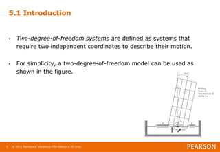
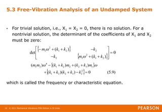
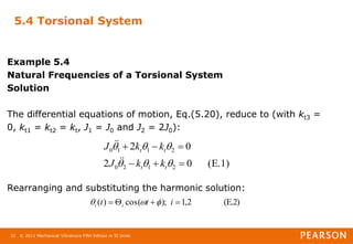
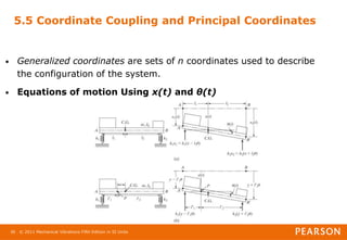
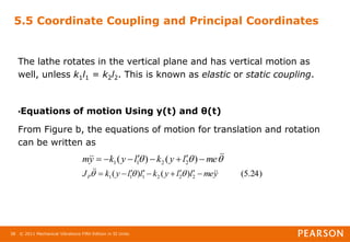
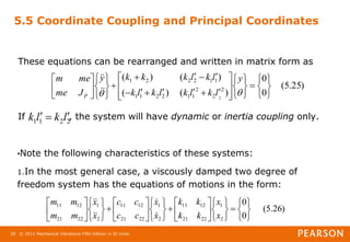
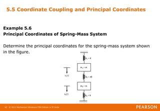
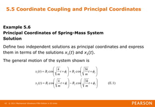
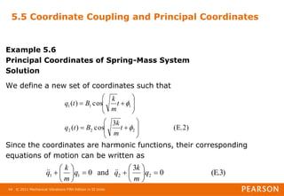
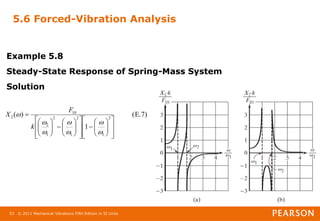
5.5 Coordinate Coupling and Principal Coordinates
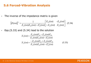
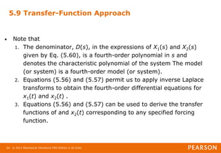
Example 5.6
Principal Coordinates of Spring-Mass System
Solution
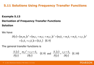
From Eqs.(E.1) and (E.2), we can write
The solution of Eqs.(E.4) gives the principal coordinates:
(E.4)
)
(
)
(
)
(
)
(
)
(
)
(
2
1
2
2
1
1
t
q
t
q
t
x
t
q
t
q
t
x




(E.5)
)]
(
)
(
[
2
1
)
(
)]
(
)
(
[
2
1
)
(
2
1
2
2
1
1
t
x
t
x
t
q
t
x
t
x
t
q





46. © 2011 Mechanical Vibrations Fifth Edition in SI Units
46
5.6
Forced-Vibration Analysis

47. © 2011 Mechanical Vibrations Fifth Edition in SI Units
47
5.6 Forced-Vibration Analysis
• The equations of motion of a general two-degree-of-freedom
system under external forces can be written as
• Consider the external forces to be harmonic:
where ω is the forcing frequency.
• We can write the steady-state solutions as
)
27
.
5
(
2
1
2
1
22
21
12
11
2
1
22
21
12
11
2
1
22
12
12
11













































F
F
x
x
k
k
k
k
x
x
c
c
c
c
x
x
m
m
m
m






)
28
.
5
(
2
,
1
,
)
( 0 
 j
e
F
t
F t
i
j
j

)
29
.
5
(
2
,
1
,
)
( 
 j
e
X
t
x t
i
j
j


48. © 2011 Mechanical Vibrations Fifth Edition in SI Units
48
5.6 Forced-Vibration Analysis
• We can write Eq.(5.30) as:
where
• Eq.(5.32) can be solved to obtain:
  )
32
.
5
(
)
( 0
F
X
i
Z




 






















20
10
0
2
1
22
12
12
11
matrix
Impedance
)
(
)
(
)
(
)
(
)
(
F
F
F
X
X
X
i
Z
i
Z
i
Z
i
Z
i
Z







  )
33
.
5
(
)
( 0
1
F
i
Z
X

 
 

49. © 2011 Mechanical Vibrations Fifth Edition in SI Units
49
5.6 Forced-Vibration Analysis
• The inverse of the impedance matrix is given
• Eqs.(5.33) and (5.34) lead to the solution
  )
34
.
5
(
)
(
)
(
)
(
)
(
)
(
)
(
)
(
1
)
(
11
12
12
22
2
12
22
11
1


















i
Z
i
Z
i
-Z
i
Z
i
Z
i
Z
i
Z
i
Z
)
35
.
5
(
)
(
)
(
)
(
)
(
)
(
)
(
)
(
)
(
)
(
)
(
)
(
)
(
2
12
22
11
20
11
10
12
2
2
12
22
11
20
12
10
22
1












i
Z
i
Z
i
Z
F
i
Z
F
i
Z
i
X
i
Z
i
Z
i
Z
F
i
Z
F
i
Z
i
X








50. © 2011 Mechanical Vibrations Fifth Edition in SI Units
50
5.6 Forced-Vibration Analysis
Example 5.8
Steady-State Response of Spring-Mass System
Find the steady-state response of system shown in Fig.5.15 when the
mass m1 is excited by the force F1(t) = F10 cos ωt. Also, plot its
frequency response curve.

51. © 2011 Mechanical Vibrations Fifth Edition in SI Units
51
5.6 Forced-Vibration Analysis
Example 5.8
Steady-State Response of Spring-Mass System
Solution
The equations of motion of the system can be expressed as
We assume the solution to be as follows
Eq.(5.31) gives
(E.1)
0
cos
2
2
0
0 10
2
1
2
1































 t
F
x
x
k
-k
-k
k
x
x
m
m 




E.2)
(
2
,
1
;
cos
)
( 
 j
t
X
t
x j
j 
(E.3)
)
(
,
2
)
(
)
( 12
2
22
11 k
Z
k
m
Z
Z 




 




52. © 2011 Mechanical Vibrations Fifth Edition in SI Units
52
5.6 Forced-Vibration Analysis
Example 5.8
Steady-State Response of Spring-Mass System
Solution
Hence
Eqs.(E.4) and (E.5) can be expressed as
(E.5)
)
)(
3
(
)
2
(
)
(
(E.4)
)
)(
3
(
)
2
(
)
2
(
)
2
(
)
(
2
2
10
2
2
2
10
2
2
2
10
2
2
2
2
10
2
1
k
m
k
m
kF
k
k
m
kF
X
k
m
k
m
F
k
m
k
k
m
F
k
m
X
































E.6)
(
1
2
)
( 2
1
2
1
2
1
2
10
2
1
1







































































k
F
X

53. © 2011 Mechanical Vibrations Fifth Edition in SI Units
53
5.6 Forced-Vibration Analysis
Example 5.8
Steady-State Response of Spring-Mass System
Solution
E.7)
(
1
)
( 2
1
2
1
2
1
2
10
2


















































k
F
X

54. © 2011 Mechanical Vibrations Fifth Edition in SI Units
54
5.7
Semidefinite Systems

55. © 2011 Mechanical Vibrations Fifth Edition in SI Units
55
5.7 Semidefinite Systems
• Semidefinite systems are also known as unrestrained or degenerate
systems.
• Two examples of such systems are shown in the figure. For Figure
(a), the equations of motion can be written as
• For free vibration, we assume the motion to be harmonic:
• Substituting Eq.(5.37) into Eq.(5.36) gives
)
36
.
5
(
0
)
(
0
)
(
1
2
2
2
2
1
1
1






x
x
k
x
m
x
x
k
x
m




)
37
.
5
(
2
,
1
),
cos(
)
( 

 j
t
X
t
x j
j
j 

)
38
.
5
(
0
)
(
0
)
(
2
2
2
1
2
1
2
1









X
k
m
kX
kX
X
k
m



56. © 2011 Mechanical Vibrations Fifth Edition in SI Units
56
5.7 Semidefinite Systems

57. © 2011 Mechanical Vibrations Fifth Edition in SI Units
57
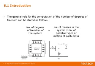
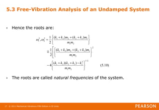
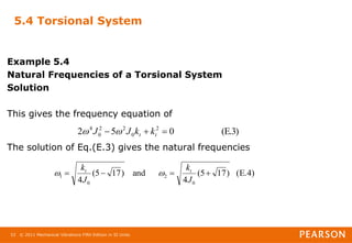
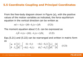
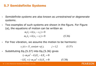
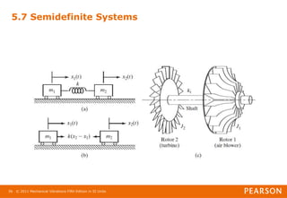
5.7 Semidefinite Systems
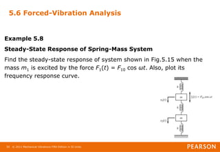
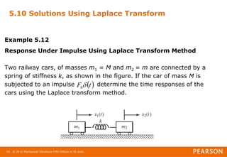
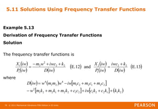
• We obtain the frequency equation as
• From which the natural frequencies can be obtained:
• Such systems, which have one of the natural frequencies equal to
zero, are called semidefinite systems.
)
39
.
5
(
0
)]
(
[ 2
1
2
2
1
2


 m
m
k
m
m 

)
40
.
5
(
)
(
and
0
2
1
2
1
2
1
m
m
m
m
k 

 


58. © 2011 Mechanical Vibrations Fifth Edition in SI Units
58
5.8
Self-Excitation and Stability Analysis

59. © 2011 Mechanical Vibrations Fifth Edition in SI Units
59
5.8 Self-Excitation and Stability Analysis
• Given that the criterion for stability is that the real parts of si must
be negative, all coefficients of equation ai must be positive and
hence, the condition
must be fulfilled.
• The Routh-Hurwitz criterion states that the system will be stable if
all the coefficients a0, a1,…,a4 are positive and the determinants
defined below are positive:
)
46
.
5
(
2
1
4
2
3
0
3
2
1 a
a
a
a
a
a
a 


60. © 2011 Mechanical Vibrations Fifth Edition in SI Units
60
5.8 Self-Excitation and Stability Analysis
)
49
.
5
(
0
0
0
)
48
.
5
(
0
)
47
.
5
(
0
2
3
0
4
2
1
3
2
1
3
1
4
2
0
3
1
3
3
0
2
1
2
0
3
1
2
1
1











a
a
a
a
a
a
a
a
a
a
a
a
a
a
T
a
a
a
a
a
a
a
a
T
a
T

61. © 2011 Mechanical Vibrations Fifth Edition in SI Units
61
5.9
Transfer-Function Approach

62. © 2011 Mechanical Vibrations Fifth Edition in SI Units
62
5.9 Transfer-Function Approach
• For two-degree-of-freedom system shown the equations of motion
are
• By taking the Laplace transforms of Eqs. (5.50) and (5.51),
assuming zero initial conditions,
     
     
5.51
5.50
2
1
2
2
3
2
1
2
2
3
2
2
2
1
2
2
1
2
1
2
2
1
2
1
1
1
f
x
k
x
k
k
x
c
x
c
c
x
m
f
x
k
x
k
k
x
c
x
c
c
x
m






















                 
                 
5.53
5.52
2
1
2
2
3
2
1
2
2
3
2
2
2
2
1
2
2
1
2
1
2
2
1
2
1
1
2
1
s
F
s
X
k
s
X
k
k
s
sX
c
s
sX
c
c
s
X
s
m
s
F
s
X
k
s
X
k
k
s
sX
c
s
sX
c
c
s
X
s
m















63. © 2011 Mechanical Vibrations Fifth Edition in SI Units
63
5.9 Transfer-Function Approach
• It can be solved using Cramer’s rule as
where
   
 
     
 
 
5.57
and
5.56 2
2
1
1
s
D
s
D
s
X
s
D
s
D
s
X 


64. © 2011 Mechanical Vibrations Fifth Edition in SI Units
64
5.9 Transfer-Function Approach
• Note that
1. The denominator, D(s), in the expressions of X1(s) and X2(s)
given by Eq. (5.60), is a fourth-order polynomial in s and
denotes the characteristic polynomial of the system The model
(or system) is a fourth-order model (or system).
2. Equations (5.56) and (5.57) permit us to apply inverse Laplace
transforms to obtain the fourth-order differential equations for
x1(t) and x2(t) .
3. Equations (5.56) and (5.57) can be used to derive the transfer
functions of and x2(t) corresponding to any specified forcing
function.

65. © 2011 Mechanical Vibrations Fifth Edition in SI Units
65
5.10
Solutions Using Laplace Transform

66. © 2011 Mechanical Vibrations Fifth Edition in SI Units
66
5.10 Solutions Using Laplace Transform
Example 5.12
Response Under Impulse Using Laplace Transform Method
Two railway cars, of masses m1 = M and m2 = m are connected by a
spring of stiffness k, as shown in the figure. If the car of mass M is
subjected to an impulse determine the time responses of the
cars using the Laplace transform method.
 
t
F 
0

67. © 2011 Mechanical Vibrations Fifth Edition in SI Units
67
5.10 Solutions Using Laplace Transform
Example 5.12
Response Under Impulse Using Laplace Transform Method
Solution
The responses of the cars can be determined using either of the
following approaches:
a. Consider the system to be undergoing free vibration due to the
initial velocity caused by the impulse applied to car M.
b. Consider the system to be undergoing forced vibration due to the
force applied to car M (with the displacements and velocities
of cars M and m considered to be zero initially).
 
t
F 
0

68. © 2011 Mechanical Vibrations Fifth Edition in SI Units
68
5.10 Solutions Using Laplace Transform
Example 5.12
Response Under Impulse Using Laplace Transform Method
Solution
Using the second approach, the equations of motion of the cars can be
expressed as
Using the Laplace transforms, Eqs. (E.1) and (E.2) can be written as
     
   
E.2
0
E.1
1
2
2
0
2
1
1






x
x
k
x
m
t
F
x
x
k
x
M



 
       
       
E.4
0
E.3
2
2
1
0
2
1
2







s
X
k
ms
s
kX
F
s
kX
s
X
k
Ms

69. © 2011 Mechanical Vibrations Fifth Edition in SI Units
69
5.10 Solutions Using Laplace Transform
Example 5.12
Response Under Impulse Using Laplace Transform Method
Solution
Equations (E.3) and (E.4) can be solved as
   
 
   
 
 
   
E.6
E.5
2
2
0
2
2
2
2
0
1
m
M
k
Mms
s
k
F
s
X
m
M
k
Mms
s
k
ms
F
s
X








70. © 2011 Mechanical Vibrations Fifth Edition in SI Units
70
5.10 Solutions Using Laplace Transform
Example 5.12
Response Under Impulse Using Laplace Transform Method
Solution
Using partial fractions, Eqs. (E.5) and (E.6) can be rewritten as
where
   
   
E.8
1
1
E.7
1
2
2
2
0
2
2
2
2
0
1




















w
s
w
w
s
m
M
F
s
X
w
s
w
wM
m
s
m
M
F
s
X
 
E.9
1
1
2








m
M
k
w

71. © 2011 Mechanical Vibrations Fifth Edition in SI Units
71
5.10 Solutions Using Laplace Transform
Example 5.12
Response Under Impulse Using Laplace Transform Method
Solution
The inverse transforms of Eqs. (E.7) and (E.8), using the results of
Appendix D, yield the time responses of the cars as
   
   
E.11
sin
1
E.10
sin
0
2
0
1


















wt
w
t
m
M
F
s
X
wt
wM
m
t
m
M
F
s
x

72. © 2011 Mechanical Vibrations Fifth Edition in SI Units
72
5.11
Solutions Using Frequency Transfer Functions

73. © 2011 Mechanical Vibrations Fifth Edition in SI Units
73
5.11 Solutions Using Frequency Transfer Functions
Example 5.13
Derivation of Frequency Transfer Functions
Derive the frequency transfer functions of x1(t) and x2(t) for the
system shown in figure.

74. © 2011 Mechanical Vibrations Fifth Edition in SI Units
74
5.11 Solutions Using Frequency Transfer Functions
Example 5.13
Derivation of Frequency Transfer Functions
Solution
From the free-body diagrams of the masses, the equations of motion
of the system is
     
     
E.2
0
E.1
sin
2
1
2
2
1
2
2
2
2
0
1
2
1
2
2
1
2
1
1
1
1
1
1














p
x
x
k
x
x
c
x
m
wt
P
p
x
x
k
x
x
c
x
k
x
c
x
m










75. © 2011 Mechanical Vibrations Fifth Edition in SI Units
75
5.11 Solutions Using Frequency Transfer Functions
Example 5.13
Derivation of Frequency Transfer Functions
Solution
By taking the Laplace transforms of Eqs. (E.1) and (E.2), assuming
zero initial conditions,
         
     
     
     
     
   
E.4
0
E.3
1
2
2
1
2
2
2
2
1
2
1
2
2
1
2
1
1
1
1
1
2
1












s
X
s
X
k
s
X
s
X
c
s
X
m
s
P
s
X
s
X
k
s
X
s
X
c
s
X
k
s
sX
c
s
X
s
m

76. © 2011 Mechanical Vibrations Fifth Edition in SI Units
76
5.11 Solutions Using Frequency Transfer Functions
Example 5.13
Derivation of Frequency Transfer Functions
Solution
The of Eqs. (E.3) and (E.4) is
where
   
 
     
 
 
E.6
and
E.5 2
2
1
1
s
D
s
D
s
X
s
D
s
D
s
X 

       
       
E.7
E.7
1
2
2
2
1
2
2
2
2
1
s
P
k
s
c
s
D
s
P
k
s
c
s
m
s
D






77. © 2011 Mechanical Vibrations Fifth Edition in SI Units
77
5.11 Solutions Using Frequency Transfer Functions
Example 5.13
Derivation of Frequency Transfer Functions
Solution
We have
The general transfer functions is
       
     
E.9
2
1
1
2
2
1
2
2
1
2
2
1
2
2
1
3
2
2
1
2
2
1
4
2
2
k
k
s
k
c
k
c
s
c
c
k
m
k
m
k
m
s
c
m
c
m
c
m
s
m
m
s
D











 
   
   
   
 
E.10
and
E.9 2
2
1
2
2
2
2
2
1
1
s
D
k
s
c
s
P
s
X
s
D
k
s
c
s
m
s
P
s
X 





78. © 2011 Mechanical Vibrations Fifth Edition in SI Units
78
5.11 Solutions Using Frequency Transfer Functions
Example 5.13
Derivation of Frequency Transfer Functions
Solution
The frequency transfer functions is
where
 
   
   
   
 
E.13
and
E.12 2
2
1
2
2
2
2
2
1
1
iw
D
k
iwc
iw
P
iw
X
iw
D
k
iwc
w
m
iw
P
iw
X 





     
     
2
1
1
2
2
1
2
1
2
2
1
2
2
1
2
2
2
1
2
2
1
4
2
1
4
k
k
k
c
k
c
iw
c
c
k
m
k
m
k
m
w
c
m
c
m
c
m
iw
w
m
m
w
iw
D










