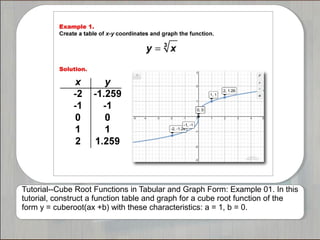
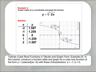
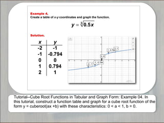
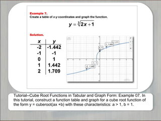
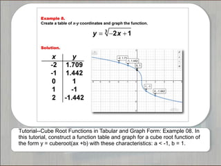
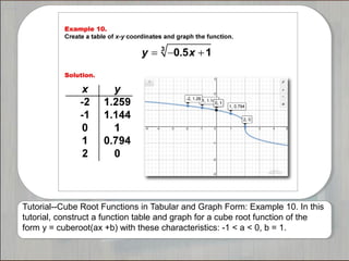
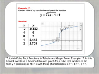
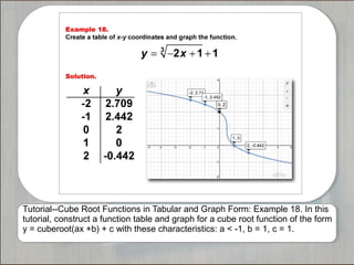
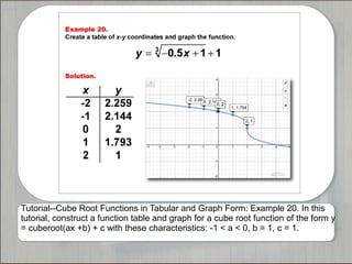
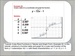
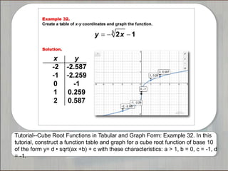
This document provides 40 examples of tutorials that construct function tables and graphs for cube root functions of the form y=cuberoot(ax+b)+c. Each tutorial varies the values of a, b, and c to illustrate different forms of cube root functions.

1. Cube Root Functions in Tabular
and Graph Form

2. Overview
This set of tutorials provides 40 examples of cube
root functions in tabular and graph form.

3. Tutorial--Cube Root Functions in Tabular and Graph Form: Example 01. In this
tutorial, construct a function table and graph for a cube root function of the
form y = cuberoot(ax +b) with these characteristics: a = 1, b = 0.

4. Tutorial--Square Root Functions in Tabular and Graph Form: Example 02. In this
tutorial, construct a function table and graph for a square root function of the form y
= sqrt(ax +b) with these characteristics: a > 1, b = 0.

5. Tutorial--Cube Root Functions in Tabular and Graph Form: Example 03. In
this tutorial, construct a function table and graph for a cube root function of
the form y = cuberoot(ax +b) with these characteristics: a < -1, b = 0.

6. Tutorial--Cube Root Functions in Tabular and Graph Form: Example 04. In
this tutorial, construct a function table and graph for a cube root function of the
form y = cuberoot(ax +b) with these characteristics: 0 < a < 1, b = 0.

7. Tutorial--Cube Root Functions in Tabular and Graph Form: Example 05. In
this tutorial, construct a function table and graph for a cube root function of
the form y = cuberoot(ax +b) with these characteristics: -1 < a < 0, b = 0.

8. Tutorial--Cube Root Functions in Tabular and Graph Form: Example 06. In
this tutorial, construct a function table and graph for a cube root function of
the form y = cuberoot(ax +b) with these characteristics: a = 1, b = 1.

9. Tutorial--Cube Root Functions in Tabular and Graph Form: Example 07. In
this tutorial, construct a function table and graph for a cube root function of
the form y = cuberoot(ax +b) with these characteristics: a > 1, b = 1.

10. Tutorial--Cube Root Functions in Tabular and Graph Form: Example 08. In
this tutorial, construct a function table and graph for a cube root function of
the form y = cuberoot(ax +b) with these characteristics: a < -1, b = 1.

11. Tutorial--Cube Root Functions in Tabular and Graph Form: Example 09. In this
tutorial, construct a function table and graph for a cube root function of the
form y = cuberoot(ax +b) with these characteristics: 0 < a < 1, b = 1.

12. Tutorial--Cube Root Functions in Tabular and Graph Form: Example 10. In this
tutorial, construct a function table and graph for a cube root function of the
form y = cuberoot(ax +b) with these characteristics: -1 < a < 0, b = 1.

13. Tutorial--Cube Root Functions in Tabular and Graph Form: Example 11. In this
tutorial, construct a function table and graph for a cube root function of the form
y = cuberoot(ax +b) + c with these characteristics: a = 1, b = 0, c = 1.

14. Tutorial--Cube Root Functions in Tabular and Graph Form: Example 12. In this
tutorial, construct a function table and graph for a cube root function of the
form y = cuberoot(ax +b) + c with these characteristics: a > 1, b = 0, c = 1.

15. Tutorial--Cube Root Functions in Tabular and Graph Form: Example 13. In this
tutorial, construct a function table and graph for a cube root function of the
form y = cuberoot(ax +b) + c with these characteristics: a < -1, b = 0, c = 1.

16. Tutorial--Cube Root Functions in Tabular and Graph Form: Example 14. In this
tutorial, construct a function table and graph for a cube root function of the form y
= cuberoot(ax +b) + c with these characteristics: 0 < a < 1, b = 0, c = 1.

17. Tutorial--Cube Root Functions in Tabular and Graph Form: Example 15. In this
tutorial, construct a function table and graph for a cube root function of the form y
= cuberoot(ax +b) + c with these characteristics: -1 < a < 0, b = 0, c = 1.

18. Tutorial--Cube Root Functions in Tabular and Graph Form: Example 16. In this
tutorial, construct a function table and graph for a cube root function of the
form y = cuberoot(ax +b) + c with these characteristics: a = 1, b = 1, c = 1.

19. Tutorial--Cube Root Functions in Tabular and Graph Form: Example 17. In this
tutorial, construct a function table and graph for a cube root function of the
form y = cuberoot(ax +b) + c with these characteristics: a > 1, b = 1, c = 1.

20. Tutorial--Cube Root Functions in Tabular and Graph Form: Example 18. In this
tutorial, construct a function table and graph for a cube root function of the form
y = cuberoot(ax +b) + c with these characteristics: a < -1, b = 1, c = 1.

21. Tutorial--Cube Root Functions in Tabular and Graph Form: Example 19. In this
tutorial, construct a function table and graph for a cube root function of the form y
= cuberoot(ax +b) + c with these characteristics: 0 < a < 1, b = 1, c = 1.

22. Tutorial--Cube Root Functions in Tabular and Graph Form: Example 20. In this
tutorial, construct a function table and graph for a cube root function of the form y
= cuberoot(ax +b) + c with these characteristics: -1 < a < 0, b = 1, c = 1.

23. Tutorial--Cube Root Functions in Tabular and Graph Form: Example 21. In this
tutorial, construct a function table and graph for a cube root function of the form
y = cuberoot(ax +b) + c with these characteristics: a = 1, b = 0, c = -1.

24. Tutorial--Cube Root Functions in Tabular and Graph Form: Example 22. In this
tutorial, construct a function table and graph for a cube root function of the
form y = cuberoot(ax +b) + c with these characteristics: a > 1, b = 0, c = -1.

25. Tutorial--Cube Root Functions in Tabular and Graph Form: Example 23. In this
tutorial, construct a function table and graph for a cube root function of the form
y = cuberoot(ax +b) + c with these characteristics: a < -1, b = 0, c = -1.

26. Tutorial--Cube Root Functions in Tabular and Graph Form: Example 24. In this
tutorial, construct a function table and graph for a cube root function of the form y
= cuberoot(ax +b) + c with these characteristics: 0 < a < 1, b = 0, c = -1.

27. Tutorial--Cube Root Functions in Tabular and Graph Form: Example 25. In this
tutorial, construct a function table and graph for a cube root function of the form
y = cuberoot(ax +b) + c with these characteristics: -1 < a < 0, b = 0, c = -1.

28. Tutorial--Cube Root Functions in Tabular and Graph Form: Example 26. In this
tutorial, construct a function table and graph for a cube root function of the
form y = cuberoot(ax +b) + c with these characteristics: a = 1, b = 1, c = -1.

29. Tutorial--Cube Root Functions in Tabular and Graph Form: Example 27. In this
tutorial, construct a function table and graph for a cube root function of the
form y = cuberoot(ax +b) + c with these characteristics: a > 1, b = 1, c = -1.

30. Tutorial--Cube Root Functions in Tabular and Graph Form: Example 28. In this
tutorial, construct a function table and graph for a cube root function of the form
y = cuberoot(ax +b) + c with these characteristics: a < -1, b = 1, c = -1.

31. Tutorial--Cube Root Functions in Tabular and Graph Form: Example 29. In this
tutorial, construct a function table and graph for a cube root function of the form y
= cuberoot(ax +b) + c with these characteristics: 0 < a < 1, b = 1, c = -1.

32. Tutorial--Cube Root Functions in Tabular and Graph Form: Example 30. In this
tutorial, construct a function table and graph for a cube root function of the form
y = cuberoot(ax +b) + c with these characteristics: -1 < a < 0, b = 1, c = -1.

33. Tutorial--Cube Root Functions in Tabular and Graph Form: Example 31. In this
tutorial, construct a function table and graph for a cube root function of base 10
of the form y= d • sqrt(ax +b) + c with these characteristics: a = 1, b = 0, c = -1, d
= -1.

34. Tutorial--Cube Root Functions in Tabular and Graph Form: Example 32. In this
tutorial, construct a function table and graph for a cube root function of base 10
of the form y= d • sqrt(ax +b) + c with these characteristics: a > 1, b = 0, c = -1, d
= -1.

35. Tutorial--Cube Root Functions in Tabular and Graph Form: Example 33. In this
tutorial, construct a function table and graph for a cube root function of base 10
of the form y= d • sqrt(ax +b) + c with these characteristics: a < -1, b = 0, c = -1,
d = -1.

36. Tutorial--Cube Root Functions in Tabular and Graph Form: Example 34. In this tutorial,
construct a function table and graph for a cube root function of base 10 of the form y= d •
sqrt(ax +b) + c with these characteristics: 0 < a < 1, b = 0, c = -1, d = -1.

37. Tutorial--Cube Root Functions in Tabular and Graph Form: Example 35. In this
tutorial, construct a function table and graph for a cube root function of base 10
of the form y= d • sqrt(ax +b) + c with these characteristics: -1 < a < 0, b = 0, c
= -1, d = -1.

38. Tutorial--Cube Root Functions in Tabular and Graph Form: Example 36. In this
tutorial, construct a function table and graph for a cube root function of base 10
of the form y= d • sqrt(ax +b) + c with these characteristics: a = 1, b = 1, c = -1,
d = -1.

39. Tutorial--Cube Root Functions in Tabular and Graph Form: Example 37. In this
tutorial, construct a function table and graph for a cube root function of base 10
of the form y= d • sqrt(ax +b) + c with these characteristics: a > 1, b = 1, c = -1,
d = -1.

40. Tutorial--Cube Root Functions in Tabular and Graph Form: Example 38. In this
tutorial, construct a function table and graph for a cube root function of base 10
of the form y= d • sqrt(ax +b) + c with these characteristics: a < -1, b = 1, c = -1,
d = -1.

41. Tutorial--Cube Root Functions in Tabular and Graph Form: Example 39. In this
tutorial, construct a function table and graph for a cube root function of base 10
of the form y= d • sqrt(ax +b) + c with these characteristics: 0 < a < 1, b = 1, c =
-1, d = -1.

42. Tutorial--Cube Root Functions in Tabular and Graph Form: Example 40. In this
tutorial, construct a function table and graph for a cube root function of base 10
of the form y= d • sqrt(ax +b) + c with these characteristics: -1 < a < 0, b = 1, c
= -1, d = -1.