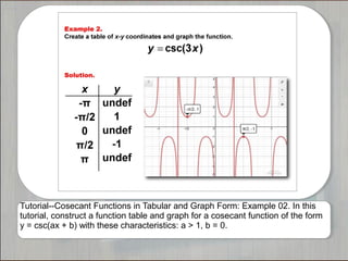
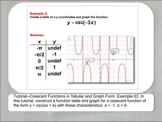
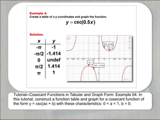
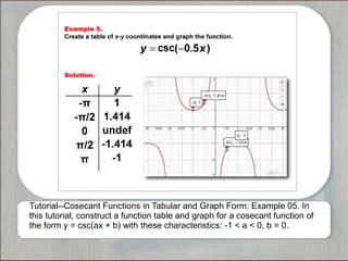
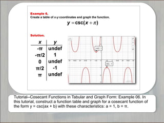
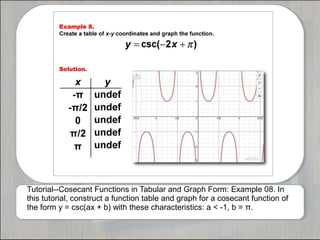
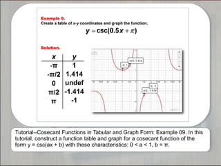
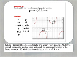
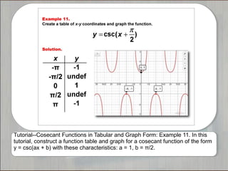
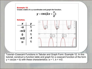
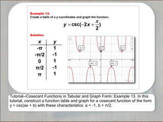
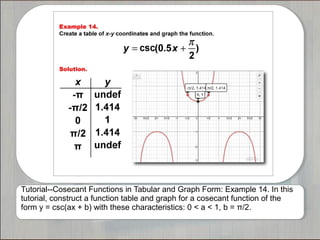
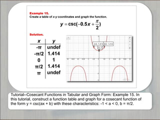
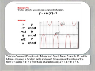
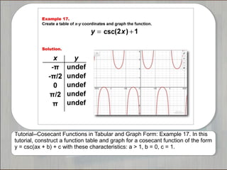
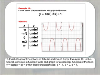
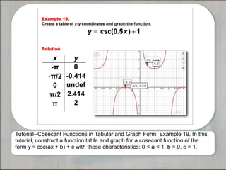
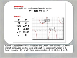
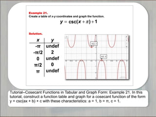
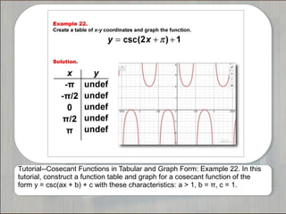
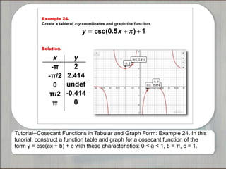
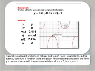
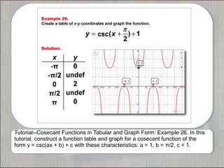
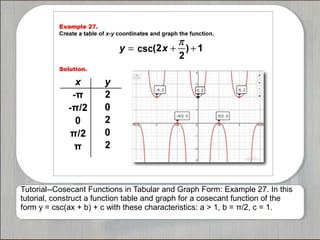
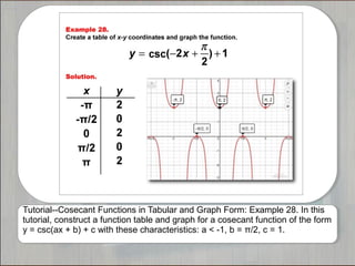
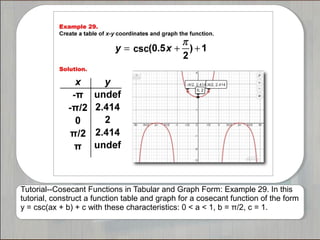
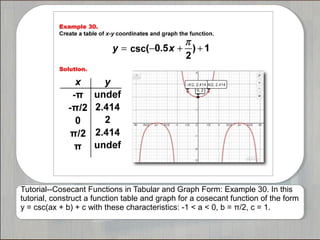
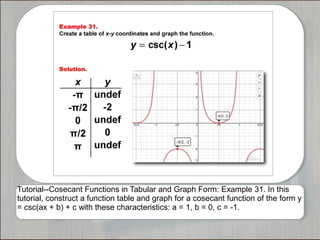
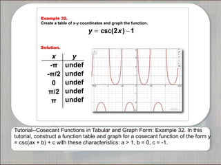
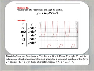
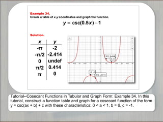
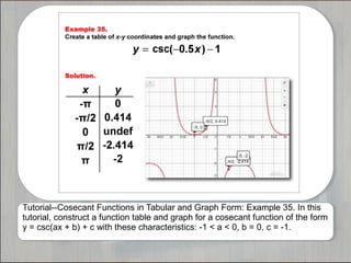
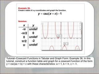
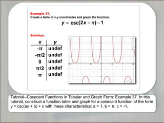
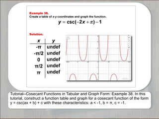
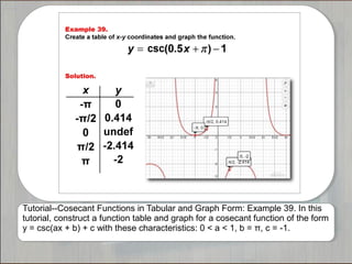
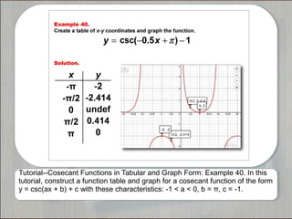
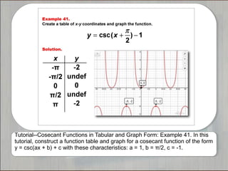
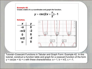
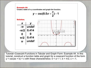
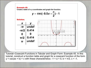
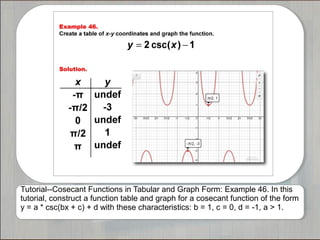
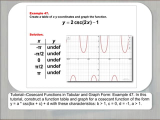
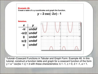
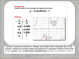
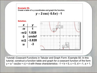
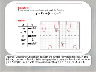
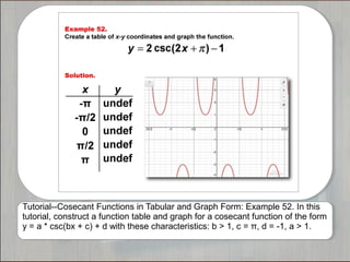
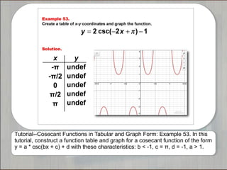
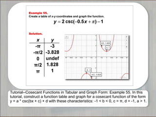
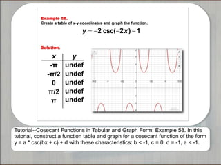
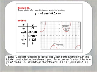
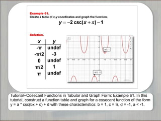
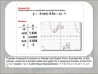
This document describes 65 tutorials that provide examples of constructing tables and graphs for cosecant functions. Each tutorial examines a cosecant function of the form y = csc(ax + b) or y = a * csc(bx + c) + d with different values for the variables a, b, c, and d. The tutorials demonstrate how changing the values of these variables affects the shape of the cosecant function graph and its table of values.
SAMPLE QUESTIONExercise 1 Consider the functionf (x,C).docxagnesdcarey33086
SAMPLE QUESTION:
Exercise 1: Consider the function
f (x,C)=
sin(C x)
Cx
(a) Create a vector x with 100 elements from -3*pi to 3*pi. Write f as an inline or anonymous function
and generate the vectors y1 = f(x,C1), y2 = f(x,C2) and y3 = f(x,C3), where C1 = 1, C2 = 2 and
C3 = 3. Make sure you suppress the output of x and y's vectors. Plot the function f (for the three
C's above), name the axis, give a title to the plot and include a legend to identify the plots. Add a
grid to the plot.
(b) Without using inline or anonymous functions write a function+function structure m-file that does
the same job as in part (a)
SAMPLE LAB WRITEUP:
MAT 275 MATLAB LAB 1 NAME: __________________________
LAB DAY and TIME:______________
Instructor: _______________________
Exercise 1
(a)
x = linspace(-3*pi,3*pi); % generating x vector - default value for number
% of pts linspace is 100
f= @(x,C) sin(C*x)./(C*x) % C will be just a constant, no need for ".*"
C1 = 1, C2 = 2, C3 = 3 % Using commans to separate commands
y1 = f(x,C1); y2 = f(x,C2); y3 = f(x,C3); % supressing the y's
plot(x,y1,'b.-', x,y2,'ro-', x,y3,'ks-') % using different markers for
% black and white plots
xlabel('x'), ylabel('y') % labeling the axis
title('f(x,C) = sin(Cx)/(Cx)') % adding a title
legend('C = 1','C = 2','C = 3') % adding a legend
grid on
Command window output:
f =
@(x,C)sin(C*x)./(C*x)
C1 =
1
C2 =
2
C3 =
3
(b)
M-file of structure function+function
function ex1
x = linspace(-3*pi,3*pi); % generating x vector - default value for number
% of pts linspace is 100
C1 = 1, C2 = 2, C3 = 3 % Using commans to separate commands
y1 = f(x,C1); y2 = f(x,C2); y3 = f(x,C3); % function f is defined below
plot(x,y1,'b.-', x,y2,'ro-', x,y3,'ks-') % using different markers for
% black and white plots
xlabel('x'), ylabel('y') % labeling the axis
title('f(x,C) = sin(Cx)/(Cx)') % adding a title
legend('C = 1','C = 2','C = 3') % adding a legend
grid on
end
function y = f(x,C)
y = sin(C*x)./(C*x);
end
Command window output:
C1 =
1
C2 =
2
C3 =
3
Joe Bob
Mon lab: 4:30-6:50
Lab 3
Exercise 1
(a) Create function M-file for banded LU factorization
function [L,U] = luband(A,p)
% LUBAND Banded LU factorization
% Adaptation to LUFACT
% Input:
% A diagonally dominant square matrix
% Output:
% L,U unit lower triangular and upper triangular such that LU=A
n = length(A);
L = eye(n); % ones on diagonal
% Gaussian Elimination
for j = 1:n-1
a = min(j+p.
M166Calculus” ProjectDue Wednesday, December 9, 2015PROJ.docxinfantsuk
M166
“Calculus” Project
Due: Wednesday, December 9, 2015
PROJECT WORTH 50 POINTS –
1) NO LATE SUBMISSIONS WILL BE ACCEPTED
2) COMPLETED PROJECTS NEED TO BE LEGIBLE
I. Computing Derivatives (slope of curve at a point) of polynomial functions.
For each of the following functions in a.-e. below perform the following three steps:
1. compute the difference quotient
2. simplify expression from part 1. such that h has been canceled from the denominator
3. substitute and simplify
a.
b.
c.
d.
e. consider , using the results from parts a. through d.,
f. find a general formula for (steps 1 through 3 performed).
II. Show that
Consider the unit circle with in standard position in QI.
a. show that the area of the right triangle (see diagram) is
b. show that the area of the sector (see diagram) is
c. show that the area of the acute triangle (see diagram)
d. set up the inequality
e. multiply the inequality in part d. by . (direction of inequalities is unchanged)
f. take the reciprocal of each term from part e. The direction of the inequality must be reversed because .
g. plug in 0 for for only. The result should be
III. Show that
a. multiply by
b. use trigonometric identity to rewrite the numerator of the expression in part a. in terms of
c. factor the expression in part b. with one factor equal to . (find remaining factor).
d. use the fact that and substitute in the second factor (result is 0)
IV. Show that derivative of
a. find the difference quotient for
(use sum angle formula )
b. factor out of the two terms in the numerator with in part a
c. split up the expression in part b with each term over the denominator h
d. use identities to simplify part c. to
Thus you have shown that if .
0
=
h
c
x
f
=
)
(
b
ax
x
f
+
=
)
(
c
bx
ax
x
f
+
+
=
2
)
(
d
cx
bx
ax
x
f
+
+
+
=
2
3
)
(
(
)
3
2
2
3
3
3
3
:
int
h
xh
h
x
x
h
x
H
+
+
+
=
+
0
1
1
1
.....
)
(
a
x
a
x
a
x
a
x
f
n
n
n
n
+
+
+
+
=
-
-
0
)
(
)
(
)
(
®
-
+
=
h
as
h
x
f
h
x
f
x
f
0
1
sin
®
=
q
q
q
as
q
2
tan
q
=
Triangle
Right
Area
2
q
=
Sector
Area
2
sin
q
=
Triangle
Acute
Area
2
sin
2
2
tan
q
q
q
³
³
q
sin
2
b
a
b
a
b
a
if
1
1
0
,
<
®
<
®
>
q
q
cos
0
1
sin
1
®
£
£
q
q
q
as
0
0
cos
1
®
=
-
q
q
q
as
q
q
cos
1
-
q
q
cos
1
cos
1
+
+
1
sin
cos
2
2
=
+
q
q
q
2
sin
q
q
sin
0
1
sin
®
=
q
q
q
as
0
=
q
q
q
cos
sin
=
h
f
h
f
f
)
(
)
(
)
(
q
q
q
-
+
=
(
)
q
q
sin
=
f
(
)
h
h
h
sin
cos
cos
sin
sin
q
q
q
+
=
+
q
sin
q
sin
0
0
cos
1
1
sin
®
=
-
=
h
as
h
h
and
h
h
q
cos
h
x
f
h
x
f
x
f
)
(
)
(
)
(
-
+
=
q
q
q
q
q
q
cos
0
)
(
)
(
)
(
,
sin
)
(
=
®
-
+
=
=
h
as
h
f
h
f
f
then
f
MATH133: Unit 3 Individual Project 2B Student Answer Form
Name (Required): ____Michael Magro_________________________
Please show all work details with answers, insert the graph, and provide answers to all the critical thinking questions on this form for the Unit 3 IP assignment.
A version of Amdah ...
MATLAB sessions: Laboratory 2
MAT 275 Laboratory 2
Matrix Computations and Programming in MATLAB
In this laboratory session we will learn how to
1. Create and manipulate matrices and vectors.
2. Write simple programs in MATLAB
NOTE: For your lab write-up, follow the instructions of LAB1.
Matrices and Linear Algebra
⋆ Matrices can be constructed in MATLAB in different ways. For example the 3 × 3 matrix
A =
8 1 63 5 7
4 9 2
can be entered as
>> A=[8,1,6;3,5,7;4,9,2]
A =
8 1 6
3 5 7
4 9 2
or
>> A=[8,1,6;
3,5,7;
4,9,2]
A =
8 1 6
3 5 7
4 9 2
or defined as the concatenation of 3 rows
>> row1=[8,1,6]; row2=[3,5,7]; row3=[4,9,2]; A=[row1;row2;row3]
A =
8 1 6
3 5 7
4 9 2
or 3 columns
>> col1=[8;3;4]; col2=[1;5;9]; col3=[6;7;2]; A=[col1,col2,col3]
A =
8 1 6
3 5 7
4 9 2
Note the use of , and ;. Concatenated rows/columns must have the same length. Larger matrices can
be created from smaller ones in the same way:
c⃝2011 Stefania Tracogna, SoMSS, ASU
MATLAB sessions: Laboratory 2
>> C=[A,A] % Same as C=[A A]
C =
8 1 6 8 1 6
3 5 7 3 5 7
4 9 2 4 9 2
The matrix C has dimension 3 × 6 (“3 by 6”). On the other hand smaller matrices (submatrices) can
be extracted from any given matrix:
>> A(2,3) % coefficient of A in 2nd row, 3rd column
ans =
7
>> A(1,:) % 1st row of A
ans =
8 1 6
>> A(:,3) % 3rd column of A
ans =
6
7
2
>> A([1,3],[2,3]) % keep coefficients in rows 1 & 3 and columns 2 & 3
ans =
1 6
9 2
⋆ Some matrices are already predefined in MATLAB:
>> I=eye(3) % the Identity matrix
I =
1 0 0
0 1 0
0 0 1
>> magic(3)
ans =
8 1 6
3 5 7
4 9 2
(what is magic about this matrix?)
⋆ Matrices can be manipulated very easily in MATLAB (unlike Maple). Here are sample commands
to exercise with:
>> A=magic(3);
>> B=A’ % transpose of A, i.e, rows of B are columns of A
B =
8 3 4
1 5 9
6 7 2
>> A+B % sum of A and B
ans =
16 4 10
4 10 16
10 16 4
>> A*B % standard linear algebra matrix multiplication
ans =
101 71 53
c⃝2011 Stefania Tracogna, SoMSS, ASU
MATLAB sessions: Laboratory 2
71 83 71
53 71 101
>> A.*B % coefficient-wise multiplication
ans =
64 3 24
3 25 63
24 63 4
⋆ One MATLAB command is especially relevant when studying the solution of linear systems of dif-
ferentials equations: x=A\b determines the solution x = A−1b of the linear system Ax = b. Here is an
example:
>> A=magic(3);
>> z=[1,2,3]’ % same as z=[1;2;3]
z =
1
2
3
>> b=A*z
b =
28
34
28
>> x = A\b % solve the system Ax = b. Compare with the exact solution, z, defined above.
x =
1
2
3
>> y =inv(A)*b % solve the system using the inverse: less efficient and accurate
ans =
1.0000
2.0000
3.0000
Now let’s check for accuracy by evaluating the difference z − x and z − y. In exact arithmetic they
should both be zero since x, y and z all represent the solution to the system.
>> z - x % error for backslash command
ans =
0
0
0
>> z - y % error for inverse
ans =
1.0e-015 *
-0.4441
0
-0.88 ...
Lab 5 template Lab 5 - Your Name - MAT 275 Lab The M.docxsmile790243
Lab 5 template
%% Lab 5 - Your Name - MAT 275 Lab
% The Mass-Spring System
%% EX 1 10 pts
%A) 1 pts | short comment
%
%B) 2 pts | short comment
%
%C) 1 pts | short comment
%
%D) 1 pts
%E) 2 pts | List the first 3-4 t values either in decimal format or as
%fractions involving pi
%F) 3 pts | comments. | (1 pts for including two distinct graphs, each with y(t) and v(t) plotted)
%% EX 2 10 pts
%A) 5 pts
% add commands to LAB05ex1 to compute and plot E(t). Then use ylim([~,~]) to change the yaxis limits.
% You don't need to include this code but at least one plot of E(t) and a comment must be
% included!
%B) 2 pts | write out main steps here
% first differentiate E(t) with respect to t using the chain rule. Then
% make substitutions using the expression for omega0 and using the
% differential equation
%C) 3 pts | show plot and comment
%% EX 3 10 pts
%A) 3 pts | modify the system of equations in LAB05ex1a
% write the t value and either a) show correponding graph or b) explain given matlab
% commands
%B) 2 pts | write t value and max |V| value; include figure
%note: velocity magnitude is like absolute value!
%C) 3 pts | include 3 figures here + comments.
% use title('text') to attach a title to the figure
%D) 2 pts | What needs to happen (in terms of the characteristic equation)
%in order for there to be no oscillations? Impose a condition on the
%characteristic equation to find the critical c value. Write out main steps
%% EX4 10 pts
% A) 5 pts | include 1 figure and comment
%B) 2 pts
% again find dE/dt using the chain rule and make substitutions based on the
% differential equation. You should reach an expression for dE/dt which is
% in terms of y'
%C) 3 pts | include one figure and comment
Exercise (1):
function LAB05ex1
m = 1; % mass [kg]
k = 9; % spring constant [N/m]
omega0=sqrt(k/m);
y0=0.4; v0=0; % initial conditions
[t,Y]=ode45(@f,[0,10],[y0,v0],[],omega0); % solve for 0<t<10
y=Y(:,1); v=Y(:,2); % retrieve y, v from Y
figure(1); plot(t,y,'b+-',t,v,'ro-'); % time series for y and v
grid on;
%------------------------------------------------------
function dYdt= f(t,Y,omega0)
y = Y(1); v= Y(2);
dYdt = [v; -omega0^2*y];
Exercise (1a):
function LAB05ex1a
m = 1; % mass [kg]
k = 9; % spring constant [N/m]
c = 1; % friction coefficient [Ns/m]
omega0 = sqrt(k/m); p = c/(2*m);
y0 = 0.4; v0 = 0; % initial conditions
[t,Y]=ode45(@f,[0,10],[y0,v0],[],omega0,p); % solve for 0<t<10
y=Y(:,1); v=Y(:,2); % retrieve y, v from Y
figure(1); plot(t,y,'b+-',t,v,'ro-'); % time series for y and v
grid on
%------------------------------------------------------
function dYdt= f(t,Y,omega0,p)
y = Y(1); v= Y(2);
dYdt = [v; ?? ]; % fill-in dv/dt
More instructions for the l ...
A hands-on activity for explore a variety of math topics, including:
* Circumference and Diameter
* Linear functions and slope
* Ratios
* Data gathering and scatterplot
For more math resources, go to www.media4math.com.
Tutorials--The Language of Math--Variable Expressions--Multiplication and Sub...Media4math
This set of tutorials provides 32 examples of converting verbal expressions into variable expressions that involve multiplication and subtraction. Note: The download is a PPT file.
Tutorials--The Language of Math--Numerical Expressions--Multiplication Media4math
This set of tutorials provides 40 examples of converting verbal expressions into numerical expressions that involve multiplication. Note: The download is a PPT file.
Tutorials--The Language of Math--Numerical Expressions--Division Media4math
This set of tutorials provides 40 examples of converting verbal expressions into numerical expressions that involve division. Note: The download is a PPT file.
Tutorials--The Language of Math--Numerical Expressions--SubtractionMedia4math
This set of tutorials provides 40 examples of converting verbal expressions into numerical expressions that involve subtraction. Note: The download is a PPT file.
Tutorials--Language of Math--Numerical Expressions--AdditionMedia4math
This set of tutorials provides 40 examples of converting verbal expressions into numerical expressions that involve addition. The verbal expressions include these terms:
Plus
Increased by
In addition to
Added to
More than
In this issue of Math in the News we explore logarithmic functions to model the thawing of frozen turkeys. We look at USDA guidelines to determine data points and use a graphing calculator to create mathematical models.
The Roman Empire A Historical Colossus.pdfkaushalkr1407
The Roman Empire, a vast and enduring power, stands as one of history's most remarkable civilizations, leaving an indelible imprint on the world. It emerged from the Roman Republic, transitioning into an imperial powerhouse under the leadership of Augustus Caesar in 27 BCE. This transformation marked the beginning of an era defined by unprecedented territorial expansion, architectural marvels, and profound cultural influence.
The empire's roots lie in the city of Rome, founded, according to legend, by Romulus in 753 BCE. Over centuries, Rome evolved from a small settlement to a formidable republic, characterized by a complex political system with elected officials and checks on power. However, internal strife, class conflicts, and military ambitions paved the way for the end of the Republic. Julius Caesar’s dictatorship and subsequent assassination in 44 BCE created a power vacuum, leading to a civil war. Octavian, later Augustus, emerged victorious, heralding the Roman Empire’s birth.
Under Augustus, the empire experienced the Pax Romana, a 200-year period of relative peace and stability. Augustus reformed the military, established efficient administrative systems, and initiated grand construction projects. The empire's borders expanded, encompassing territories from Britain to Egypt and from Spain to the Euphrates. Roman legions, renowned for their discipline and engineering prowess, secured and maintained these vast territories, building roads, fortifications, and cities that facilitated control and integration.
The Roman Empire’s society was hierarchical, with a rigid class system. At the top were the patricians, wealthy elites who held significant political power. Below them were the plebeians, free citizens with limited political influence, and the vast numbers of slaves who formed the backbone of the economy. The family unit was central, governed by the paterfamilias, the male head who held absolute authority.
Culturally, the Romans were eclectic, absorbing and adapting elements from the civilizations they encountered, particularly the Greeks. Roman art, literature, and philosophy reflected this synthesis, creating a rich cultural tapestry. Latin, the Roman language, became the lingua franca of the Western world, influencing numerous modern languages.
Roman architecture and engineering achievements were monumental. They perfected the arch, vault, and dome, constructing enduring structures like the Colosseum, Pantheon, and aqueducts. These engineering marvels not only showcased Roman ingenuity but also served practical purposes, from public entertainment to water supply.
Synthetic Fiber Construction in lab .pptxPavel ( NSTU)
Synthetic fiber production is a fascinating and complex field that blends chemistry, engineering, and environmental science. By understanding these aspects, students can gain a comprehensive view of synthetic fiber production, its impact on society and the environment, and the potential for future innovations. Synthetic fibers play a crucial role in modern society, impacting various aspects of daily life, industry, and the environment. ynthetic fibers are integral to modern life, offering a range of benefits from cost-effectiveness and versatility to innovative applications and performance characteristics. While they pose environmental challenges, ongoing research and development aim to create more sustainable and eco-friendly alternatives. Understanding the importance of synthetic fibers helps in appreciating their role in the economy, industry, and daily life, while also emphasizing the need for sustainable practices and innovation.
Unit 8 - Information and Communication Technology (Paper I).pdfThiyagu K
This slides describes the basic concepts of ICT, basics of Email, Emerging Technology and Digital Initiatives in Education. This presentations aligns with the UGC Paper I syllabus.
How to Create Map Views in the Odoo 17 ERPCeline George
The map views are useful for providing a geographical representation of data. They allow users to visualize and analyze the data in a more intuitive manner.
Instructions for Submissions thorugh G- Classroom.pptxJheel Barad
This presentation provides a briefing on how to upload submissions and documents in Google Classroom. It was prepared as part of an orientation for new Sainik School in-service teacher trainees. As a training officer, my goal is to ensure that you are comfortable and proficient with this essential tool for managing assignments and fostering student engagement.
The Art Pastor's Guide to Sabbath | Steve ThomasonSteve Thomason
What is the purpose of the Sabbath Law in the Torah. It is interesting to compare how the context of the law shifts from Exodus to Deuteronomy. Who gets to rest, and why?
Ethnobotany and Ethnopharmacology:
Ethnobotany in herbal drug evaluation,
Impact of Ethnobotany in traditional medicine,
New development in herbals,
Bio-prospecting tools for drug discovery,
Role of Ethnopharmacology in drug evaluation,
Reverse Pharmacology.
2024.06.01 Introducing a competency framework for languag learning materials ...Sandy Millin
http://sandymillin.wordpress.com/iateflwebinar2024
Published classroom materials form the basis of syllabuses, drive teacher professional development, and have a potentially huge influence on learners, teachers and education systems. All teachers also create their own materials, whether a few sentences on a blackboard, a highly-structured fully-realised online course, or anything in between. Despite this, the knowledge and skills needed to create effective language learning materials are rarely part of teacher training, and are mostly learnt by trial and error.
Knowledge and skills frameworks, generally called competency frameworks, for ELT teachers, trainers and managers have existed for a few years now. However, until I created one for my MA dissertation, there wasn’t one drawing together what we need to know and do to be able to effectively produce language learning materials.
This webinar will introduce you to my framework, highlighting the key competencies I identified from my research. It will also show how anybody involved in language teaching (any language, not just English!), teacher training, managing schools or developing language learning materials can benefit from using the framework.
Palestine last event orientationfvgnh .pptxRaedMohamed3
An EFL lesson about the current events in Palestine. It is intended to be for intermediate students who wish to increase their listening skills through a short lesson in power point.
2. Overview
This set of tutorials provides 65 examples of
cosecant functions in tabular and graph form.
3. Tutorial--Cosecant Functions in Tabular and Graph Form: Example 01. In this
tutorial, construct a function table and graph for a cosecant function of the form
y = csc(ax + b) with these characteristics: a = 1, b = 0.
4. Tutorial--Cosecant Functions in Tabular and Graph Form: Example 02. In this
tutorial, construct a function table and graph for a cosecant function of the form
y = csc(ax + b) with these characteristics: a > 1, b = 0.
5. Tutorial--Cosecant Functions in Tabular and Graph Form: Example 03. In
this tutorial, construct a function table and graph for a cosecant function of
the form y = csc(ax + b) with these characteristics: a < -1, b = 0.
6. Tutorial--Cosecant Functions in Tabular and Graph Form: Example 04. In
this tutorial, construct a function table and graph for a cosecant function of
the form y = csc(ax + b) with these characteristics: 0 < a < 1, b = 0.
7. Tutorial--Cosecant Functions in Tabular and Graph Form: Example 05. In
this tutorial, construct a function table and graph for a cosecant function of
the form y = csc(ax + b) with these characteristics: -1 < a < 0, b = 0.
8. Tutorial--Cosecant Functions in Tabular and Graph Form: Example 06. In
this tutorial, construct a function table and graph for a cosecant function of
the form y = csc(ax + b) with these characteristics: a = 1, b = π.
9. Tutorial--Cosecant Functions in Tabular and Graph Form: Example 07. In
this tutorial, construct a function table and graph for a cosecant function of
the form y = csc(ax + b) with these characteristics: a > 1, b = π.
10. Tutorial--Cosecant Functions in Tabular and Graph Form: Example 08. In
this tutorial, construct a function table and graph for a cosecant function of
the form y = csc(ax + b) with these characteristics: a < -1, b = π.
11. Tutorial--Cosecant Functions in Tabular and Graph Form: Example 09. In this
tutorial, construct a function table and graph for a cosecant function of the
form y = csc(ax + b) with these characteristics: 0 < a < 1, b = π.
12. Tutorial--Cosecant Functions in Tabular and Graph Form: Example 10. In this
tutorial, construct a function table and graph for a cosecant function of the
form y = csc(ax + b) with these characteristics: -1 < a < 0, b = π.
13. Tutorial--Cosecant Functions in Tabular and Graph Form: Example 11. In this
tutorial, construct a function table and graph for a cosecant function of the form
y = csc(ax + b) with these characteristics: a = 1, b = π/2.
14. Tutorial--Cosecant Functions in Tabular and Graph Form: Example 12. In this
tutorial, construct a function table and graph for a cosecant function of the form
y = csc(ax + b) with these characteristics: a > 1, b = π/2.
15. Tutorial--Cosecant Functions in Tabular and Graph Form: Example 13. In this
tutorial, construct a function table and graph for a cosecant function of the form
y = csc(ax + b) with these characteristics: a < -1, b = π/2.
16. Tutorial--Cosecant Functions in Tabular and Graph Form: Example 14. In this
tutorial, construct a function table and graph for a cosecant function of the
form y = csc(ax + b) with these characteristics: 0 < a < 1, b = π/2.
17. Tutorial--Cosecant Functions in Tabular and Graph Form: Example 15. In
this tutorial, construct a function table and graph for a cosecant function of
the form y = csc(ax + b) with these characteristics: -1 < a < 0, b = π/2.
18. Tutorial--Cosecant Functions in Tabular and Graph Form: Example 16. In this
tutorial, construct a function table and graph for a cosecant function of the
form y = csc(ax + b) + c with these characteristics: a = 1, b = 0, c = 1.
19. Tutorial--Cosecant Functions in Tabular and Graph Form: Example 17. In this
tutorial, construct a function table and graph for a cosecant function of the form
y = csc(ax + b) + c with these characteristics: a > 1, b = 0, c = 1.
20. Tutorial--Cosecant Functions in Tabular and Graph Form: Example 18. In this
tutorial, construct a function table and graph for a cosecant function of the form
y = csc(ax + b) + c with these characteristics: a < -1, b = 0, c = 1.
21. Tutorial--Cosecant Functions in Tabular and Graph Form: Example 19. In this
tutorial, construct a function table and graph for a cosecant function of the
form y = csc(ax + b) + c with these characteristics: 0 < a < 1, b = 0, c = 1.
22. Tutorial--Cosecant Functions in Tabular and Graph Form: Example 20. In this
tutorial, construct a function table and graph for a cosecant function of the
form y = csc(ax + b) + c with these characteristics: -1 < a < 0, b = 0, c = 1.
23. Tutorial--Cosecant Functions in Tabular and Graph Form: Example 21. In this
tutorial, construct a function table and graph for a cosecant function of the form
y = csc(ax + b) + c with these characteristics: a = 1, b = π, c = 1.
24. Tutorial--Cosecant Functions in Tabular and Graph Form: Example 22. In this
tutorial, construct a function table and graph for a cosecant function of the
form y = csc(ax + b) + c with these characteristics: a > 1, b = π, c = 1.
25. Tutorial--Cosecant Functions in Tabular and Graph Form: Example 23. In this
tutorial, construct a function table and graph for a cosecant function of the
form y = csc(ax + b) + c with these characteristics: a < -1, b = π, c = 1.
26. Tutorial--Cosecant Functions in Tabular and Graph Form: Example 24. In this
tutorial, construct a function table and graph for a cosecant function of the
form y = csc(ax + b) + c with these characteristics: 0 < a < 1, b = π, c = 1.
27. Tutorial--Cosecant Functions in Tabular and Graph Form: Example 25. In this
tutorial, construct a function table and graph for a cosecant function of the form
y = csc(ax + b) + c with these characteristics: -1 < a < 0, b = π, c = 1.
28. Tutorial--Cosecant Functions in Tabular and Graph Form: Example 26. In this
tutorial, construct a function table and graph for a cosecant function of the
form y = csc(ax + b) + c with these characteristics: a = 1, b = π/2, c = 1.
29. Tutorial--Cosecant Functions in Tabular and Graph Form: Example 27. In this
tutorial, construct a function table and graph for a cosecant function of the
form y = csc(ax + b) + c with these characteristics: a > 1, b = π/2, c = 1.
30. Tutorial--Cosecant Functions in Tabular and Graph Form: Example 28. In this
tutorial, construct a function table and graph for a cosecant function of the form
y = csc(ax + b) + c with these characteristics: a < -1, b = π/2, c = 1.
31. Tutorial--Cosecant Functions in Tabular and Graph Form: Example 29. In this
tutorial, construct a function table and graph for a cosecant function of the form
y = csc(ax + b) + c with these characteristics: 0 < a < 1, b = π/2, c = 1.
32. Tutorial--Cosecant Functions in Tabular and Graph Form: Example 30. In this
tutorial, construct a function table and graph for a cosecant function of the form
y = csc(ax + b) + c with these characteristics: -1 < a < 0, b = π/2, c = 1.
33. Tutorial--Cosecant Functions in Tabular and Graph Form: Example 31. In this
tutorial, construct a function table and graph for a cosecant function of the form y
= csc(ax + b) + c with these characteristics: a = 1, b = 0, c = -1.
34. Tutorial--Cosecant Functions in Tabular and Graph Form: Example 32. In this
tutorial, construct a function table and graph for a cosecant function of the form y
= csc(ax + b) + c with these characteristics: a > 1, b = 0, c = -1.
35. Tutorial--Cosecant Functions in Tabular and Graph Form: Example 33. In this
tutorial, construct a function table and graph for a cosecant function of the form
y = csc(ax + b) + c with these characteristics: a < -1, b = 0, c = -1.
36. Tutorial--Cosecant Functions in Tabular and Graph Form: Example 34. In this
tutorial, construct a function table and graph for a cosecant function of the form
y = csc(ax + b) + c with these characteristics: 0 < a < 1, b = 0, c = -1.
37. Tutorial--Cosecant Functions in Tabular and Graph Form: Example 35. In this
tutorial, construct a function table and graph for a cosecant function of the form
y = csc(ax + b) + c with these characteristics: -1 < a < 0, b = 0, c = -1.
38. Tutorial--Cosecant Functions in Tabular and Graph Form: Example 36. In this
tutorial, construct a function table and graph for a cosecant function of the form
y = csc(ax + b) + c with these characteristics: a = 1, b = π, c = -1.
39. Tutorial--Cosecant Functions in Tabular and Graph Form: Example 37. In this
tutorial, construct a function table and graph for a cosecant function of the form
y = csc(ax + b) + c with these characteristics: a > 1, b = π, c = -1.
40. Tutorial--Cosecant Functions in Tabular and Graph Form: Example 38. In this
tutorial, construct a function table and graph for a cosecant function of the form
y = csc(ax + b) + c with these characteristics: a < -1, b = π, c = -1.
41. Tutorial--Cosecant Functions in Tabular and Graph Form: Example 39. In this
tutorial, construct a function table and graph for a cosecant function of the form
y = csc(ax + b) + c with these characteristics: 0 < a < 1, b = π, c = -1.
42. Tutorial--Cosecant Functions in Tabular and Graph Form: Example 40. In this
tutorial, construct a function table and graph for a cosecant function of the form
y = csc(ax + b) + c with these characteristics: -1 < a < 0, b = π, c = -1.
43. Tutorial--Cosecant Functions in Tabular and Graph Form: Example 41. In this
tutorial, construct a function table and graph for a cosecant function of the form
y = csc(ax + b) + c with these characteristics: a = 1, b = π/2, c = -1.
44. Tutorial--Cosecant Functions in Tabular and Graph Form: Example 42. In this
tutorial, construct a function table and graph for a cosecant function of the form
y = csc(ax + b) + c with these characteristics: a > 1, b = π/2, c = -1.
45. Tutorial--Cosecant Functions in Tabular and Graph Form: Example 43. In this
tutorial, construct a function table and graph for a cosecant function of the form
y = csc(ax + b) + c with these characteristics: a < -1, b = π/2, c = -1.
46. Tutorial--Cosecant Functions in Tabular and Graph Form: Example 44. In this
tutorial, construct a function table and graph for a cosecant function of the form
y = csc(ax + b) + c with these characteristics: 0 < a < 1, b = π/2, c = -1.
47. Tutorial--Cosecant Functions in Tabular and Graph Form: Example 45. In this
tutorial, construct a function table and graph for a cosecant function of the form
y = csc(ax + b) + c with these characteristics: -1 < a < 0, b = π/2, c = -1.
48. Tutorial--Cosecant Functions in Tabular and Graph Form: Example 46. In this
tutorial, construct a function table and graph for a cosecant function of the form
y = a * csc(bx + c) + d with these characteristics: b = 1, c = 0, d = -1, a > 1.
49. Tutorial--Cosecant Functions in Tabular and Graph Form: Example 47. In this
tutorial, construct a function table and graph for a cosecant function of the form
y = a * csc(bx + c) + d with these characteristics: b > 1, c = 0, d = -1, a > 1.
50. Tutorial--Cosecant Functions in Tabular and Graph Form: Example 48. In this
tutorial, construct a function table and graph for a cosecant function of the form
y = a * csc(bx + c) + d with these characteristics: b < -1, c = 0, d = -1, a > 1.
51. Tutorial--Cosecant Functions in Tabular and Graph Form: Example 49. In this
tutorial, construct a function table and graph for a cosecant function of the form
y = a * csc(bx + c) + d with these characteristics: 0 < b < 1, c = 0, d = -1, a > 1.
52. Tutorial--Cosecant Functions in Tabular and Graph Form: Example 50. In this
tutorial, construct a function table and graph for a cosecant function of the form
y = a * csc(bx + c) + d with these characteristics: -1 < b < 0, c = 0, d = -1, a > 1.
53. Tutorial--Cosecant Functions in Tabular and Graph Form: Example 51. In this
tutorial, construct a function table and graph for a cosecant function of the form
y = a * csc(bx + c) + d with these characteristics: b = 1, c = π, d= -1, a > 1.
54. Tutorial--Cosecant Functions in Tabular and Graph Form: Example 52. In this
tutorial, construct a function table and graph for a cosecant function of the form
y = a * csc(bx + c) + d with these characteristics: b > 1, c = π, d = -1, a > 1.
55. Tutorial--Cosecant Functions in Tabular and Graph Form: Example 53. In this
tutorial, construct a function table and graph for a cosecant function of the form
y = a * csc(bx + c) + d with these characteristics: b < -1, c = π, d = -1, a > 1.
56. Tutorial--Cosecant Functions in Tabular and Graph Form: Example 54. In this
tutorial, construct a function table and graph for a cosecant function of the form
y = a * csc(bx + c) + d with these characteristics: 0 < b < 1, c = π, d = -1, a > 1.
57. Tutorial--Cosecant Functions in Tabular and Graph Form: Example 55. In this
tutorial, construct a function table and graph for a cosecant function of the form
y = a * csc(bx + c) + d with these characteristics: -1 < b < 0, c = π, d = -1, a > 1.
58. Tutorial--Cosecant Functions in Tabular and Graph Form: Example 56. In this
tutorial, construct a function table and graph for a cosecant function of the form
y = a * csc(bx + c) + d with these characteristics: b = 1, c = 0, d = -1, a < -1.
59. Tutorial--Cosecant Functions in Tabular and Graph Form: Example 57. In this
tutorial, construct a function table and graph for a cosecant function of the form
y = a * csc(bx + c) + d with these characteristics: b > 1, c = 0, d = -1, a < -1.
60. Tutorial--Cosecant Functions in Tabular and Graph Form: Example 58. In this
tutorial, construct a function table and graph for a cosecant function of the form
y = a * csc(bx + c) + d with these characteristics: b < -1, c = 0, d = -1, a < -1.
61. Tutorial--Cosecant Functions in Tabular and Graph Form: Example 59. In this
tutorial, construct a function table and graph for a cosecant function of the form
y = a * csc(bx + c) + d with these characteristics: 0 < b < 1, c = 0, d = -1, a < -1.
62. Tutorial--Cosecant Functions in Tabular and Graph Form: Example 60. In this
tutorial, construct a function table and graph for a cosecant function of the form
y = a * csc(bx + c) + d with these characteristics: -1 < b < 0, c = 0, d = -1, a <
-1.
63. Tutorial--Cosecant Functions in Tabular and Graph Form: Example 61. In this
tutorial, construct a function table and graph for a cosecant function of the form
y = a * csc(bx + c) + d with these characteristics: b = 1, c = π, d = -1, a < -1.
64. Tutorial--Cosecant Functions in Tabular and Graph Form: Example 62. In this
tutorial, construct a function table and graph for a cosecant function of the form
y = a * csc(bx + c) + d with these characteristics: b > 1, c = π, d = -1, a < -1.
65. Tutorial--Cosecant Functions in Tabular and Graph Form: Example 63. In this
tutorial, construct a function table and graph for a cosecant function of the form
y = a * csc(bx + c) + d with these characteristics: b < -1, c = π, d = -1, e < -1.
66. Tutorial--Cosecant Functions in Tabular and Graph Form: Example 64. In this
tutorial, construct a function table and graph for a cosecant function of the form
y = a * csc(bx + c) + d with these characteristics: 0 < b < 1, c = π, d = -1, a < -1.
67. Tutorial--Cosecant Functions in Tabular and Graph Form: Example 65. In this
tutorial, construct a function table and graph for a cosecant function of the form
y = a * csc(bx + c) + d with these characteristics: -1 < b < 0, c = π, d = -1, a <
-1.