Download as PDF, PPTX


![Green Wireless Communications
• Green Information & Communications Tech. (ICT) [1]
– the 5th largest industry in power consumption
– energy consumption: 3% (2007’)
– CO2 emission: 2% (2007’) will increase X35, 4% (2020’)
– e.g., cellular networks:
ƒ energy: 77.5 TWh (2/60/3.5/10 TWh for 3b/4MM/20,000/etc.
subscribers/radio stations/radio controllers/others)
ƒ CO2: 35 Mt (1/20/2/5 Mt for “ )
Jingon Joung Tutorial 2: Energy Efficient Wireless Communications 5 / 112](https://image.slidesharecdn.com/tutorialiceic2015-150603000145-lva1-app6892/85/Energy-Efficient-Wireless-Communications-6-320.jpg)
![Green Wireless Communications
• Wireless access communication networks consume
significant amount of energy to overcome [2]
– fading, distortion, degradation (path loss)
– obstacles, interferences
TX
wirelesschannel
RX
Jingon Joung Tutorial 2: Energy Efficient Wireless Communications 5 / 112](https://image.slidesharecdn.com/tutorialiceic2015-150603000145-lva1-app6892/85/Energy-Efficient-Wireless-Communications-7-320.jpg)
![Green Wireless Communications
• The energy is mostly consumed at the
transmitter
• e.g., 80-85% power at base station (BS) in
cellular networks [2]
Base Band
Module
D
A
C
Informationbinarybits
Filter Filter
LO
LFTPA
Attn. control
DC control
Mixer
VGA
Synthethesizer
Jingon Joung Tutorial 2: Energy Efficient Wireless Communications 5 / 112](https://image.slidesharecdn.com/tutorialiceic2015-150603000145-lva1-app6892/85/Energy-Efficient-Wireless-Communications-8-320.jpg)
![Green Wireless Communications
• 50–80% of transmitter’s power is
consumed at power amplifier (PA) [3]
PA
input
signal
output
signal
DC
Jingon Joung Tutorial 2: Energy Efficient Wireless Communications 5 / 112](https://image.slidesharecdn.com/tutorialiceic2015-150603000145-lva1-app6892/85/Energy-Efficient-Wireless-Communications-9-320.jpg)
![References
[1]:
[McK, 2007]
[Fettweis and Zimmermann, 2008]
[Mancuso and Sara Alouf, 2011]
[Chatzipapas et al., 2011]
[2]:
[Richter et al., 2009]
[Baliga et al., 2011]
[Vereecken et al., 2011]
[Chatzipapas et al., 2011]
[Joung and Sun, 2012]
[3]:
[Gruber et al., 2009]
[Bogucka and Conti, 2011]
[Joung et al., 2012a]
[Joung et al., 2014c]
[Joung et al., 2013]
Jingon Joung Tutorial 2: Energy Efficient Wireless Communications 6 / 112](https://image.slidesharecdn.com/tutorialiceic2015-150603000145-lva1-app6892/85/Energy-Efficient-Wireless-Communications-10-320.jpg)


![Efficiency in Communications
valuable resource produced in comm: information, coverage, subscribers, ...
valuable resource consumed in comm: frequency, space, time, power, ...
Spectral Efficiency (SE) and Energy Efficiency (EE)
SE, b/s/Hz: number of reliably decoded bits per channel use
[Cover and Thomas, 2006, Verd´u, 2002, Chen et al., 2011]
- Shannon (channel) capacity, data rate (throughput), goodput
EE, b/J: number of reliably decoded bits per energy
- various EEs in communications
Jingon Joung Tutorial 2: Energy Efficient Wireless Communications 10 / 112](https://image.slidesharecdn.com/tutorialiceic2015-150603000145-lva1-app6892/85/Energy-Efficient-Wireless-Communications-16-320.jpg)
![Efficiency in Communications
valuable resource produced in comm: information, coverage, subscribers, ...
valuable resource consumed in comm: frequency, space, time, power, ...
Spectral Efficiency (SE) and Energy Efficiency (EE)
SE, b/s/Hz: number of reliably decoded bits per channel use
[Cover and Thomas, 2006, Verd´u, 2002, Chen et al., 2011]
- Shannon (channel) capacity, data rate (throughput), goodput
EE, b/J: number of reliably decoded bits per energy
- various EEs in communications
Jingon Joung Tutorial 2: Energy Efficient Wireless Communications 10 / 112](https://image.slidesharecdn.com/tutorialiceic2015-150603000145-lva1-app6892/85/Energy-Efficient-Wireless-Communications-17-320.jpg)
![Efficiency in Communications
valuable resource produced in comm: information, coverage, subscribers, ...
valuable resource consumed in comm: frequency, space, time, power, ...
Spectral Efficiency (SE) and Energy Efficiency (EE)
SE, b/s/Hz: number of reliably decoded bits per channel use
[Cover and Thomas, 2006, Verd´u, 2002, Chen et al., 2011]
- Shannon (channel) capacity, data rate (throughput), goodput
EE, b/J: number of reliably decoded bits per energy
- various EEs in communications
Jingon Joung Tutorial 2: Energy Efficient Wireless Communications 10 / 112](https://image.slidesharecdn.com/tutorialiceic2015-150603000145-lva1-app6892/85/Energy-Efficient-Wireless-Communications-18-320.jpg)
![Various EEs in Comms.
Table 1: Various EEs [Richter et al., 2009, Tombaz et al., 2011, Hasan et al., 2011,
Zhou et al., 2013, Joung et al., ].
Metric Type Units
power usage efficiency facility-level ratio (≥ 1)
data center efficiency facility-level %
telecommun. energy effi. ratio equipment-level Gbps/W
telecommun. equipment energy effi. rating equipment-level − log(Gbps/W)
energy consumption rating equipment-level W/Gbps
area power consumption network-level Km2
/W
user power consumption network-level users/W
network energy effi. with delay effect network-level dB/J
pecuniary efficiency network-level bits/$
Jingon Joung Tutorial 2: Energy Efficient Wireless Communications 11 / 112](https://image.slidesharecdn.com/tutorialiceic2015-150603000145-lva1-app6892/85/Energy-Efficient-Wireless-Communications-19-320.jpg)

![Theoretical SE-EE Tradeoff
SE, b/s/Hz
EE,b/J
Figure 1: Theoretical SE-EE tradeoff. Figure 2: Ideal power consumption.
SE = log2(1 + Pout/σ2
): Gaussian signalling, perfectly linear PA
[Cover and Thomas, 2006]
EE = Ω SE
Pc
: ideal power consumption model in Fig. 2
[Verd´u, 2002, Chen et al., 2011]
[Pout: transmit power; σ2: noise power; Ω: total bandwidth]
Convex and wide (good) tradeoff
Jingon Joung Tutorial 2: Energy Efficient Wireless Communications 13 / 112](https://image.slidesharecdn.com/tutorialiceic2015-150603000145-lva1-app6892/85/Energy-Efficient-Wireless-Communications-21-320.jpg)
![Theoretical SE-EE Tradeoff
SE, b/s/Hz
EE,b/J
Figure 1: Theoretical SE-EE tradeoff.
Pc PPA Pout==
Figure 2: Ideal power consumption.
SE = log2(1 + Pout/σ2
): Gaussian signalling, perfectly linear PA
[Cover and Thomas, 2006]
EE = Ω SE
Pc
: ideal power consumption model in Fig. 2
[Verd´u, 2002, Chen et al., 2011]
[Pout: transmit power; σ2: noise power; Ω: total bandwidth]
Convex and wide (good) tradeoff
Jingon Joung Tutorial 2: Energy Efficient Wireless Communications 13 / 112](https://image.slidesharecdn.com/tutorialiceic2015-150603000145-lva1-app6892/85/Energy-Efficient-Wireless-Communications-22-320.jpg)
![Theoretical SE-EE Tradeoff
SE, b/s/Hz
EE,b/J
1
σ2 ln 2
Figure 1: Theoretical SE-EE tradeoff.
Pc PPA Pout==
Figure 2: Ideal power consumption.
SE = log2(1 + Pout/σ2
): Gaussian signalling, perfectly linear PA
[Cover and Thomas, 2006]
EE = Ω SE
Pc
: ideal power consumption model in Fig. 2
[Verd´u, 2002, Chen et al., 2011]
[Pout: transmit power; σ2: noise power; Ω: total bandwidth]
Convex and wide (good) tradeoff
Jingon Joung Tutorial 2: Energy Efficient Wireless Communications 13 / 112](https://image.slidesharecdn.com/tutorialiceic2015-150603000145-lva1-app6892/85/Energy-Efficient-Wireless-Communications-23-320.jpg)


![Basic Circuit Model of PA
ACRF-drive,Pin DC input, PDC
PAoutput,Pout
Power Amplifier (PA)
Figure 4: Power amplifier model with field-effect transistor (FET)
[Cripps, 2006, Kazimierczuk, 2008].
Transistor is a core semiconductor device:
amplifies and switches electronic signals and electrical power
changes a voltage or current: terminals (G,D) to terminals (S,D)
Jingon Joung Tutorial 2: Energy Efficient Wireless Communications 16 / 112](https://image.slidesharecdn.com/tutorialiceic2015-150603000145-lva1-app6892/85/Energy-Efficient-Wireless-Communications-26-320.jpg)
![Basic Circuit Model of PA
ACRF-drive,Pin
DC input, PDC
PAoutput,Pout
gate
drainsource
transistor
RFC
DC blocking capacitor
inputnetwork
outputnetwork
resistor
Figure 4: Power amplifier model with field-effect transistor (FET)
[Cripps, 2006, Kazimierczuk, 2008].
Transistor is a core semiconductor device:
amplifies and switches electronic signals and electrical power
changes a voltage or current: terminals (G,D) to terminals (S,D)
Jingon Joung Tutorial 2: Energy Efficient Wireless Communications 16 / 112](https://image.slidesharecdn.com/tutorialiceic2015-150603000145-lva1-app6892/85/Energy-Efficient-Wireless-Communications-27-320.jpg)


![Linearity Models [Teikari, 2008]
Transistor-level
System-level
accurate yet difficult to obtain, generalize or analyze
a few parameters obtained from measurements,
tractable, and reasonably accurate
PA
Linearity
Models
[23][Vuolevi et al., 2000], [24][Boumaiza and Ghannouchi, 2003], [25][Gadringer et al., 2005],
[26][Morgan et al., 2006], [27][Kim and Konstantinou, 2001], [28][Jeruchim et al., 2000]
Jingon Joung Tutorial 2: Energy Efficient Wireless Communications 19 / 112](https://image.slidesharecdn.com/tutorialiceic2015-150603000145-lva1-app6892/85/Energy-Efficient-Wireless-Communications-30-320.jpg)
![Linearity Models [Teikari, 2008]
Transistor-level
System-level
Memory Memoryless
accurate yet difficult to obtain, generalize or analyze
a few parameters obtained from measurements,
tractable, and reasonably accurate
a frequency-domain fluctuation due to
the capacitance and Inductance in the
circuits and the thermal fluctuation of
the PAs, i.e., an electrical and thermal
memory effects, respectively [23,24]
Volterra series model [25]
Wiener, Hammerstein models [26]
Memory polynomial [27]
previous PA output signal
does not affect the current
PA output signal
PA
Linearity
Models
[23][Vuolevi et al., 2000], [24][Boumaiza and Ghannouchi, 2003], [25][Gadringer et al., 2005],
[26][Morgan et al., 2006], [27][Kim and Konstantinou, 2001], [28][Jeruchim et al., 2000]
Jingon Joung Tutorial 2: Energy Efficient Wireless Communications 19 / 112](https://image.slidesharecdn.com/tutorialiceic2015-150603000145-lva1-app6892/85/Energy-Efficient-Wireless-Communications-31-320.jpg)
![Linearity Models [Teikari, 2008]
Transistor-level
System-level
Memory Memoryless Passband
Baseband
accurate yet difficult to obtain, generalize or analyze
a few parameters obtained from measurements,
tractable, and reasonably accurate
a frequency-domain fluctuation due to
the capacitance and Inductance in the
circuits and the thermal fluctuation of
the PAs, i.e., an electrical and thermal
memory effects, respectively [23,24]
Volterra series model [25]
Wiener, Hammerstein models [26]
Memory polynomial [27]
previous PA output signal
does not affect the current
PA output signal
difficult to do simulation
and computation
Nonlinearity of complex
baseband frequency
approximation is
captured simply [28]
PA
Linearity
Models
[23][Vuolevi et al., 2000], [24][Boumaiza and Ghannouchi, 2003], [25][Gadringer et al., 2005],
[26][Morgan et al., 2006], [27][Kim and Konstantinou, 2001], [28][Jeruchim et al., 2000]
Jingon Joung Tutorial 2: Energy Efficient Wireless Communications 19 / 112](https://image.slidesharecdn.com/tutorialiceic2015-150603000145-lva1-app6892/85/Energy-Efficient-Wireless-Communications-32-320.jpg)
![Memoryless Baseband PA Models
Generic model: simplified baseband model for tractable analysis
Ideal model for analysis:
y = gx,
where x and y are PA input and output signals; and g > 0 is a linear gain.
Linear model for analysis [Minkoff, 1985]:
y = gx + n,
where n is the nonlinear distortion that is independent of x and modeled as
Gaussian noise based on Bussgang’s theorem [Bussgang, 1952].
Soft limiter model for analysis [Tellado et al., 2003]: y = γ (|x|) e2πjΦ(|x|)
- γ(·): amplitude-dependent gain function
- Φ(·): phase shift function
γ (|x|)
|x|, if |x| < vsat,
vsat, otherwise,
Φ(|x|) 0
where vsat is a saturation output amplitude.
Jingon Joung Tutorial 2: Energy Efficient Wireless Communications 20 / 112](https://image.slidesharecdn.com/tutorialiceic2015-150603000145-lva1-app6892/85/Energy-Efficient-Wireless-Communications-33-320.jpg)
![Memoryless Baseband PA Models
Generic model: simplified baseband model for tractable analysis
Ideal model for analysis:
y = gx,
where x and y are PA input and output signals; and g > 0 is a linear gain.
Linear model for analysis [Minkoff, 1985]:
y = gx + n,
where n is the nonlinear distortion that is independent of x and modeled as
Gaussian noise based on Bussgang’s theorem [Bussgang, 1952].
Soft limiter model for analysis [Tellado et al., 2003]: y = γ (|x|) e2πjΦ(|x|)
- γ(·): amplitude-dependent gain function
- Φ(·): phase shift function
γ (|x|)
|x|, if |x| < vsat,
vsat, otherwise,
Φ(|x|) 0
where vsat is a saturation output amplitude.
Jingon Joung Tutorial 2: Energy Efficient Wireless Communications 20 / 112](https://image.slidesharecdn.com/tutorialiceic2015-150603000145-lva1-app6892/85/Energy-Efficient-Wireless-Communications-34-320.jpg)
![Memoryless Baseband PA Models
Generic model: simplified baseband model for tractable analysis
Ideal model for analysis:
y = gx,
where x and y are PA input and output signals; and g > 0 is a linear gain.
Linear model for analysis [Minkoff, 1985]:
y = gx + n,
where n is the nonlinear distortion that is independent of x and modeled as
Gaussian noise based on Bussgang’s theorem [Bussgang, 1952].
Soft limiter model for analysis [Tellado et al., 2003]: y = γ (|x|) e2πjΦ(|x|)
- γ(·): amplitude-dependent gain function
- Φ(·): phase shift function
γ (|x|)
|x|, if |x| < vsat,
vsat, otherwise,
Φ(|x|) 0
where vsat is a saturation output amplitude.
Jingon Joung Tutorial 2: Energy Efficient Wireless Communications 20 / 112](https://image.slidesharecdn.com/tutorialiceic2015-150603000145-lva1-app6892/85/Energy-Efficient-Wireless-Communications-35-320.jpg)
![Memoryless Baseband PA Models
Generic model: simplified baseband model for tractable analysis
Ideal model for analysis:
y = gx,
where x and y are PA input and output signals; and g > 0 is a linear gain.
Linear model for analysis [Minkoff, 1985]:
y = gx + n,
where n is the nonlinear distortion that is independent of x and modeled as
Gaussian noise based on Bussgang’s theorem [Bussgang, 1952].
Soft limiter model for analysis [Tellado et al., 2003]: y = γ (|x|) e2πjΦ(|x|)
- γ(·): amplitude-dependent gain function
- Φ(·): phase shift function
γ (|x|)
|x|, if |x| < vsat,
vsat, otherwise,
Φ(|x|) 0
where vsat is a saturation output amplitude.
Jingon Joung Tutorial 2: Energy Efficient Wireless Communications 20 / 112](https://image.slidesharecdn.com/tutorialiceic2015-150603000145-lva1-app6892/85/Energy-Efficient-Wireless-Communications-36-320.jpg)
![Memoryless Baseband PA Models
PA-specific model: accurate baseband model specified to PA type
Saleh model for traveling wave tube amplifier [Saleh, 1981]:
γ (|x|)
a1|x|
1 + a2|x|2
; Φ(|x|)
b1|x|2
1 + b2|x|2
where ai and bi are the distortion coefficients
Ghorbani model for FET PA and for low amplitude nonlinearity
[Ghorbani and Sheikhan, 1991]:
γ (|x|)
a1|xa2
|
1 + a3|xa2 |
+ a4|x|; Φ(|x|)
b1|xb2
|
1 + b3|xb2 |
+ b4|x|
Rapp model for envelope characteristic of solid state PA (especially,
class-AB) [Rapp, 1991, Falconer et al., 2000]:
γ (|x|) |x| 1 +
|x|
vsat
2p − 1
2p
; Φ(|x|) 0
where p is a smoothness factor.
Jingon Joung Tutorial 2: Energy Efficient Wireless Communications 21 / 112](https://image.slidesharecdn.com/tutorialiceic2015-150603000145-lva1-app6892/85/Energy-Efficient-Wireless-Communications-37-320.jpg)
![Memoryless Baseband PA Models
PA-specific model: accurate baseband model specified to PA type
Saleh model for traveling wave tube amplifier [Saleh, 1981]:
γ (|x|)
a1|x|
1 + a2|x|2
; Φ(|x|)
b1|x|2
1 + b2|x|2
where ai and bi are the distortion coefficients
Ghorbani model for FET PA and for low amplitude nonlinearity
[Ghorbani and Sheikhan, 1991]:
γ (|x|)
a1|xa2
|
1 + a3|xa2 |
+ a4|x|; Φ(|x|)
b1|xb2
|
1 + b3|xb2 |
+ b4|x|
Rapp model for envelope characteristic of solid state PA (especially,
class-AB) [Rapp, 1991, Falconer et al., 2000]:
γ (|x|) |x| 1 +
|x|
vsat
2p − 1
2p
; Φ(|x|) 0
where p is a smoothness factor.
Jingon Joung Tutorial 2: Energy Efficient Wireless Communications 21 / 112](https://image.slidesharecdn.com/tutorialiceic2015-150603000145-lva1-app6892/85/Energy-Efficient-Wireless-Communications-38-320.jpg)
![Memoryless Baseband PA Models
PA-specific model: accurate baseband model specified to PA type
Saleh model for traveling wave tube amplifier [Saleh, 1981]:
γ (|x|)
a1|x|
1 + a2|x|2
; Φ(|x|)
b1|x|2
1 + b2|x|2
where ai and bi are the distortion coefficients
Ghorbani model for FET PA and for low amplitude nonlinearity
[Ghorbani and Sheikhan, 1991]:
γ (|x|)
a1|xa2
|
1 + a3|xa2 |
+ a4|x|; Φ(|x|)
b1|xb2
|
1 + b3|xb2 |
+ b4|x|
Rapp model for envelope characteristic of solid state PA (especially,
class-AB) [Rapp, 1991, Falconer et al., 2000]:
γ (|x|) |x| 1 +
|x|
vsat
2p − 1
2p
; Φ(|x|) 0
where p is a smoothness factor.
Jingon Joung Tutorial 2: Energy Efficient Wireless Communications 21 / 112](https://image.slidesharecdn.com/tutorialiceic2015-150603000145-lva1-app6892/85/Energy-Efficient-Wireless-Communications-39-320.jpg)
![Memoryless Baseband PA Models
PA-specific model: accurate baseband model specified to PA type
Saleh model for traveling wave tube amplifier [Saleh, 1981]:
γ (|x|)
a1|x|
1 + a2|x|2
; Φ(|x|)
b1|x|2
1 + b2|x|2
where ai and bi are the distortion coefficients
Ghorbani model for FET PA and for low amplitude nonlinearity
[Ghorbani and Sheikhan, 1991]:
γ (|x|)
a1|xa2
|
1 + a3|xa2 |
+ a4|x|; Φ(|x|)
b1|xb2
|
1 + b3|xb2 |
+ b4|x|
Rapp model for envelope characteristic of solid state PA (especially,
class-AB) [Rapp, 1991, Falconer et al., 2000]:
γ (|x|) |x| 1 +
|x|
vsat
2p − 1
2p
; Φ(|x|) 0
where p is a smoothness factor.
Jingon Joung Tutorial 2: Energy Efficient Wireless Communications 21 / 112](https://image.slidesharecdn.com/tutorialiceic2015-150603000145-lva1-app6892/85/Energy-Efficient-Wireless-Communications-40-320.jpg)

![Efficiency Models
Efficiencies of PA [Kazimierczuk, 2008, Raab et al., 2002]
1 Drain efficiency: ηD
Pout
PDC
2 Power-added efficiency (PAE): ηPAE
Pout−Pin
PDC
= ηD 1 − 1
g
3 Overall efficiency: ηO
Pout
PDC+Pin
Typically η ηD ≃ ηPAE ≃ ηO, ∵ Pin ≪ PDC, Pin ≪ Pout
Two important factors
Jingon Joung Tutorial 2: Energy Efficient Wireless Communications 23 / 112](https://image.slidesharecdn.com/tutorialiceic2015-150603000145-lva1-app6892/85/Energy-Efficient-Wireless-Communications-42-320.jpg)
![Efficiency Models
Efficiencies of PA [Kazimierczuk, 2008, Raab et al., 2002]
1 Drain efficiency: ηD
Pout
PDC
2 Power-added efficiency (PAE): ηPAE
Pout−Pin
PDC
= ηD 1 − 1
g
3 Overall efficiency: ηO
Pout
PDC+Pin
Typically η ηD ≃ ηPAE ≃ ηO, ∵ Pin ≪ PDC, Pin ≪ Pout
Two important factors
Jingon Joung Tutorial 2: Energy Efficient Wireless Communications 23 / 112](https://image.slidesharecdn.com/tutorialiceic2015-150603000145-lva1-app6892/85/Energy-Efficient-Wireless-Communications-43-320.jpg)
![Efficiency Models
Efficiencies of PA [Kazimierczuk, 2008, Raab et al., 2002]
1 Drain efficiency: ηD
Pout
PDC
2 Power-added efficiency (PAE): ηPAE
Pout−Pin
PDC
= ηD 1 − 1
g
3 Overall efficiency: ηO
Pout
PDC+Pin
Typically η ηD ≃ ηPAE ≃ ηO, ∵ Pin ≪ PDC, Pin ≪ Pout
Two important factors
Jingon Joung Tutorial 2: Energy Efficient Wireless Communications 23 / 112](https://image.slidesharecdn.com/tutorialiceic2015-150603000145-lva1-app6892/85/Energy-Efficient-Wireless-Communications-44-320.jpg)
![PA Efficiency < 100%
5 10 15 20 25 30 35 40 45 50 55
5
10
15
20
25
30
35
40
45
50
55
20% drain efficiency line
30% drain efficiency line
100% drain efficiency line
PAs: 0−1 GHz
PAs: 1−2 GHz
PAs: 2−3 GHz
PAs: 3−4 GHz
PAs: 4−5 GHz
PDC dBm
Pout(Pmax)dBm
Figure 8: Maximum output power (at the linear region) versus PDC.
η < 100% [Raab et al., 2003a]
Typically between 20% and 30% [Joung et al., 2012a]
Jingon Joung Tutorial 2: Energy Efficient Wireless Communications 24 / 112](https://image.slidesharecdn.com/tutorialiceic2015-150603000145-lva1-app6892/85/Energy-Efficient-Wireless-Communications-45-320.jpg)
![PA Efficiency Drop
0 5 10 15 20 25 28 30 34 40 45 50
0
10
20
30
40
50
60
70
Power-addedefficiency(PAE),ǫ%
Pout dBm
SKY65162-70LF
optimal matching
Doherty
class-AB
MAX2840
RF2132
RF2146
SST13LP01
AN10923
Doherty 21180
Figure 9: PAE versus Pout.
η usually drops rapidly as the output power decreases [Shirvani et al., 2002]
a peak η is achieved at the peak envelope power (PEP)
Jingon Joung Tutorial 2: Energy Efficient Wireless Communications 25 / 112](https://image.slidesharecdn.com/tutorialiceic2015-150603000145-lva1-app6892/85/Energy-Efficient-Wireless-Communications-46-320.jpg)
![PA Classes
Table 2: Examples of PA Classes
[Raab et al., 2002, Raab et al., 2003a, Raab et al., 2003b].
Class Linearity Efficiency Utilization Factor Main Applications
A high ≤ 50% 0.125
millimeter wave (30-100GHz)
4W/30%/Ka-band
250mW/25%/Q-band
200mW/10%/W-band
B high ≤ 78.5% 0.125 broadband at HF and VHF
C ≤ 85% - high-power vacuum-tube Tx
D low ≤ 100% 0.159 100W to 1kW HF
E low ≤ 100% 0.098
high-efficiency at K-band
16W with 80% efficiency at UHF
100mW with 60% efficiency at 10GHz
F low very high ≥ 50% from 0.125 to 0.159 UHF and microwave
(operation) class: amplification method
power-output capability (transistor utilization factor):
output power
(# of transistor)×(peak drain voltage)×(peak drain current)
Jingon Joung Tutorial 2: Energy Efficient Wireless Communications 26 / 112](https://image.slidesharecdn.com/tutorialiceic2015-150603000145-lva1-app6892/85/Energy-Efficient-Wireless-Communications-47-320.jpg)
![Applications of PAs
HF VHF UHF L S C X Ku K Ka V W G THF
3M 30M 300M 1G 2G 12G 18G4G 8G 26.5G 40G 110G 300G 3T3G 75G
(1-300M)
Comm. Submarines (3-30K)
AM broadcasts (153K-26M)
Navigation
FM (87.5-108M)
TV (54M-890M, VHF, UHF)
Weather radio (162M)
Aircraft comm.
Land/maritime mobile comm.
RFID (ISM band)
Shortwave Broadcasts
Citizens' band radio
Over-the-horizon radar/comm.
Amateur radio
(3G-30G)
WLAN 802.11a/ac/ad/n (5G)
DBS (10.7G-12.75G)
Satellite comm./TV (C,Ku,Ka)
Microwave devices/communications
Modern radars
Radio astronomy
Amateur radio
(30G-300G)
LMDS (26G-29G, 31G-31.3G)
WLAN 802.11ad (60G)
HIgh-frequency microwave radio relay
MIcrowave remote sensing
DIrected-energy weapon
MIllimeter wave scanner
Radio astronomy
Amateur radio
(1T~)
Terahertz imaging
Ultrafast molecular dynamics
Condensed-matter physics
Terahertz time-domain spectroscopy
Terahertz computing/communications
Sub-mm remote sensing
Amateur radio
(300M-3G)
FRS/GMRS (462M-467M)
ZigBee (ISM: 868M,915M,2.4G)
Z-Wave (900M)
DECT/Cordless telephone (900M)
GPS (1.2,1.5G)
GSM (900M,1.8G)
UMTS (2.1G)
LTE (698M-3.8G)
WLAN (802.11b/g/n/ad 2.4G)
Bluetooth (2.4-2.483.5MHz)
BAN/WBAN/BSN (2.36G-2.4G)
UWB (1.6G-10.5G)
Modern Cordless telephone (1.9G,2.4G,5.8G)
Si LDMOS
GaN-HEMT
Si RF CMOS
SiGe-HBT, SiGe-BiCMOS
GaAs-HBT, GaAs-pHEMT
InP-HBT InP-HEMT, GaAs-mEHMT
SiC-MESFET
0
Figure 10: Power amplifier applications over IEEE bands [Joung et al., 2014b].
FET: field effect transistor
MOSFET: metal oxide semiconductor FET
MESFET: metal epitaxial semiconductor FET
DMOS: diffued metal oxide semiconductor
LDMOS: laterally DMOS
CMOS: complementary metal oxide semicond.
BiCMOS: bipolar CMOS
HBT: heterojunction bipolar transistor
HEMT: high electron mobility transistor
mHEMT: metamorphic HEMT
pHEMT: pseudomorphic HEMT
SiGe: silicon Germanium
GaAs: Gallium Arsenide
GaN: Gallium Nitride
InP: Indium Phosphide
ISM: industrial, scientific and medical
WPAN: wireless personal area network
WLAN: wireless local area network
LTE: long term evolution
GSM: Global system for mobile communications
UMTS: universal mobile telecommun. system
UWB: ultra-wide band
GPS: global positioning system
FRS: family radio service
GMRS: general mobile radio service
BSN: body sensor network
BAN: body area network
WBAN: wireless body area network
DBS: direct-broadcast satellite
LMDS: local multipoint distribution service
DECT: digital enhanced cordless telecommun.
Jingon Joung Tutorial 2: Energy Efficient Wireless Communications 27 / 112](https://image.slidesharecdn.com/tutorialiceic2015-150603000145-lva1-app6892/85/Energy-Efficient-Wireless-Communications-48-320.jpg)
![PA in Wireless Communications
The LDMOS PA are employed for many communication equipments.
The international technology roadmap for semiconductors (ITRS) reports
that 48 volt LDMOS transistor is widely used in cellular infrastructure
market in 2011 [ITRS, 2011].
∵ The LDMOS can support high output power required for a base station
(BS) in cellular networks.
Table 3: Transmit Power of BSs [Auer et al., 2011, earth, 2015]
Type Pmax
out back-off average max output power ISD [m]
Macro 54 dBm (250 W) 8 dB 43 dBm (20 W) 1 Km −5 Km
Micro 46 dBm (40 W) 8 dB 38 dBm (6.3 W) 100 m −500 m
Pico 33 dBm (2 W) 12 dB 21 dBm (125 mW) 10 m −80 m
Femto 29 dBm (800 mW) 12 dB 17 dBm (50 mW) indoor
To compensate poor efficiency of LDMOS devices in the low power regime,
envelope tracking architecture or Doherty technique is used for 3G and 4G
networks that employs high PAPR waveform signals.
Jingon Joung Tutorial 2: Energy Efficient Wireless Communications 28 / 112](https://image.slidesharecdn.com/tutorialiceic2015-150603000145-lva1-app6892/85/Energy-Efficient-Wireless-Communications-49-320.jpg)
![Previous Studies on the Practical
SE-EE Tradeoff
Practical SE analysis with PA nonlinearity for multicarrier systems
[Tellado et al., 2003, Zillmann and Fettweis, 2005,
Gutman and Wulich, 2012]
Practical SE-EE tradeoff conjecture [Chen et al., 2011]
Practical SE-EE tradeoff analysis with practical power consumption model
[H´eliot et al., 2012, Onireti et al., 2012]
Analytical and numerical quantification of SE-EE tradeoff with BOTH
nonlinearity and imperfect efficiency of PA
[Joung et al., 2012a, Joung et al., 2014c]
Jingon Joung Tutorial 2: Energy Efficient Wireless Communications 29 / 112](https://image.slidesharecdn.com/tutorialiceic2015-150603000145-lva1-app6892/85/Energy-Efficient-Wireless-Communications-50-320.jpg)
![Previous Studies on the Practical
SE-EE Tradeoff
Practical SE analysis with PA nonlinearity for multicarrier systems
[Tellado et al., 2003, Zillmann and Fettweis, 2005,
Gutman and Wulich, 2012]
Practical SE-EE tradeoff conjecture [Chen et al., 2011]
Practical SE-EE tradeoff analysis with practical power consumption model
[H´eliot et al., 2012, Onireti et al., 2012]
Analytical and numerical quantification of SE-EE tradeoff with BOTH
nonlinearity and imperfect efficiency of PA
[Joung et al., 2012a, Joung et al., 2014c]
Jingon Joung Tutorial 2: Energy Efficient Wireless Communications 29 / 112](https://image.slidesharecdn.com/tutorialiceic2015-150603000145-lva1-app6892/85/Energy-Efficient-Wireless-Communications-51-320.jpg)
![Previous Studies on the Practical
SE-EE Tradeoff
Practical SE analysis with PA nonlinearity for multicarrier systems
[Tellado et al., 2003, Zillmann and Fettweis, 2005,
Gutman and Wulich, 2012]
Practical SE-EE tradeoff conjecture [Chen et al., 2011]
Practical SE-EE tradeoff analysis with practical power consumption model
[H´eliot et al., 2012, Onireti et al., 2012]
Analytical and numerical quantification of SE-EE tradeoff with BOTH
nonlinearity and imperfect efficiency of PA
[Joung et al., 2012a, Joung et al., 2014c]
Jingon Joung Tutorial 2: Energy Efficient Wireless Communications 29 / 112](https://image.slidesharecdn.com/tutorialiceic2015-150603000145-lva1-app6892/85/Energy-Efficient-Wireless-Communications-52-320.jpg)
![Practical SE-EE Tradeoff
SE, b/s/Hz
EE,b/J
?
Figure 11: Practical SE-EE tradeoff.
Pc PPA Pout≫≫
Figure 12: Practical Power Consumption.
Practical system’s power consumption model in Fig. 12
efficiency < 100% and PA nonlinearity
SE is not a log function anymore [Joung et al., 2012a, Joung et al., 2014c]
Concave, narrow (bad), and biased tradeoff
Jingon Joung Tutorial 2: Energy Efficient Wireless Communications 30 / 112](https://image.slidesharecdn.com/tutorialiceic2015-150603000145-lva1-app6892/85/Energy-Efficient-Wireless-Communications-53-320.jpg)
![Practical SE-EE Tradeoff
SE, b/s/Hz
EE,b/J
?
Figure 11: Practical SE-EE tradeoff.
Pc PPA Pout≫≫
Figure 12: Practical Power Consumption.
Practical system’s power consumption model in Fig. 12
efficiency < 100% and PA nonlinearity
SE is not a log function anymore [Joung et al., 2012a, Joung et al., 2014c]
Concave, narrow (bad), and biased tradeoff
Jingon Joung Tutorial 2: Energy Efficient Wireless Communications 30 / 112](https://image.slidesharecdn.com/tutorialiceic2015-150603000145-lva1-app6892/85/Energy-Efficient-Wireless-Communications-54-320.jpg)
![Practical SE-EE Tradeoff
SE, b/s/Hz
EE,b/J
Theoretical tradeoff in Fig. 1
Figure 11: Practical SE-EE tradeoff.
Pc PPA Pout≫≫
Figure 12: Practical Power Consumption.
Practical system’s power consumption model in Fig. 12
efficiency < 100% and PA nonlinearity
SE is not a log function anymore [Joung et al., 2012a, Joung et al., 2014c]
Concave, narrow (bad), and biased tradeoff
Jingon Joung Tutorial 2: Energy Efficient Wireless Communications 30 / 112](https://image.slidesharecdn.com/tutorialiceic2015-150603000145-lva1-app6892/85/Energy-Efficient-Wireless-Communications-55-320.jpg)


![EE Tech. [Joung et al., 2014b]
Approaches Methods Improvement Challenges
1. PA Design
linear architecture Linearity (L)
high cost,
parallel architecture Efficiency (E)
large form factor
switching architecture (PAS) E
envelope tracking (ET) architecture E
PA circuit architecture
envelope elimination & restoration (EER/Kahn) L, E
outphasing technique (LINK) L, E
Doherty technique E
2. Signal Design
PAPR reduction
clipping
L, E
out-of-band emission
coding
additional resource,partial transmit sequence (PTS)
latency,
PA input/output
selective mapping (SLM)
complexity
signal processing
tone reservation (TR)
tone insertion (TI)
Linearlization
feed forward sensitive to PA,
feedback additional circuit,
digital predistortion (DPD) complexity
3. Network Design
Network densification
E
infrastructure,
in/out band small cells
overhead signalling,
distributed antenna system (DAS)
scalability,
Efficient network
cooperative communications (relay)
handover,
topology & protocol
Network protocol
interference
design by
cell zooming
deploying low power PA
coordinated multipoint (CoMP)
or using PA on/off
cell discontinuous TX/RX (DTX/DRX)
coordinated sleep and napping (CoNap)
Jingon Joung Tutorial 2: Energy Efficient Wireless Communications 34 / 112](https://image.slidesharecdn.com/tutorialiceic2015-150603000145-lva1-app6892/85/Energy-Efficient-Wireless-Communications-63-320.jpg)

![1. PA Design
Architecture: a building block of various circuits (e.g., multiple PAs,
oscillators, mixers, filters, matching networks, combiners, and circulators)
Transmitter Architecture: direct approach, PA package structures
1 Linear architecture [Raab et al., 2003c]
2 Corporate architecture [Cripps, 2006]
3 Parallel architecture [Shirvani et al., 2002, Alc, 2008]
4 Stage bypassing and gate switching [Raab et al., 2003c, Staudinger, 2000]
5 Envelope elimination and restoration (EER) technique (or Kahn)
[Raab et al., 2003c, Kahn, 1952]
6 Envelope tracking architecture [Raab et al., 2003c] F
7 Outphasing using linear amplification using nonlinear components (LINK)
[Raab et al., 2003c, Cox, 1974]
8 Doherty technique [Cha et al., 2004, Doherty, 1936, Correia et al., 2010,
Auer et al., 2011, Arnold et al., 2010] F
9 Combined complex architecture, etc.
Jingon Joung Tutorial 2: Energy Efficient Wireless Communications 36 / 112](https://image.slidesharecdn.com/tutorialiceic2015-150603000145-lva1-app6892/85/Energy-Efficient-Wireless-Communications-65-320.jpg)
![1. PA Design
Architecture: a building block of various circuits (e.g., multiple PAs,
oscillators, mixers, filters, matching networks, combiners, and circulators)
Transmitter Architecture: direct approach, PA package structures
1 Linear architecture [Raab et al., 2003c]
2 Corporate architecture [Cripps, 2006]
3 Parallel architecture [Shirvani et al., 2002, Alc, 2008]
4 Stage bypassing and gate switching [Raab et al., 2003c, Staudinger, 2000]
5 Envelope elimination and restoration (EER) technique (or Kahn)
[Raab et al., 2003c, Kahn, 1952]
6 Envelope tracking architecture [Raab et al., 2003c] F
7 Outphasing using linear amplification using nonlinear components (LINK)
[Raab et al., 2003c, Cox, 1974]
8 Doherty technique [Cha et al., 2004, Doherty, 1936, Correia et al., 2010,
Auer et al., 2011, Arnold et al., 2010] F
9 Combined complex architecture, etc.
Jingon Joung Tutorial 2: Energy Efficient Wireless Communications 36 / 112](https://image.slidesharecdn.com/tutorialiceic2015-150603000145-lva1-app6892/85/Energy-Efficient-Wireless-Communications-66-320.jpg)

![Key Points
Table 4: Efficiency, costs and environmental impact of a 20,000-base-station network
with different power amplifier technologies [Mancuso and Sara Alouf, 2011].
Traditional technology Doherty technology Envelope tracking
PA efficiency 15 % 25 % 45 %
Power consumption 51.7 MW 27.2 MW 16.1 MW
CO2 emission 194,600 tons 102,400 tons 60,800 tons
Power cost 54.3 MM$ 28.6 MM$ 17.0 MM$
Challenges:
Nonlinearity and inefficiency are fundamental and inevitable.
mathematical model: modeling and empirical evaluation, i.e.,
simulated-annealing-based custom computer-aided design
high manufacturing cost
large form factor
wide dynamic range with high efficiency
advanced materials and metamaterials
Jingon Joung Tutorial 2: Energy Efficient Wireless Communications 38 / 112](https://image.slidesharecdn.com/tutorialiceic2015-150603000145-lva1-app6892/85/Energy-Efficient-Wireless-Communications-68-320.jpg)
![Key Points
Table 4: Efficiency, costs and environmental impact of a 20,000-base-station network
with different power amplifier technologies [Mancuso and Sara Alouf, 2011].
Traditional technology Doherty technology Envelope tracking
PA efficiency 15 % 25 % 45 %
Power consumption 51.7 MW 27.2 MW 16.1 MW
CO2 emission 194,600 tons 102,400 tons 60,800 tons
Power cost 54.3 MM$ 28.6 MM$ 17.0 MM$
Challenges:
Nonlinearity and inefficiency are fundamental and inevitable.
mathematical model: modeling and empirical evaluation, i.e.,
simulated-annealing-based custom computer-aided design
high manufacturing cost
large form factor
wide dynamic range with high efficiency
advanced materials and metamaterials
Jingon Joung Tutorial 2: Energy Efficient Wireless Communications 38 / 112](https://image.slidesharecdn.com/tutorialiceic2015-150603000145-lva1-app6892/85/Energy-Efficient-Wireless-Communications-69-320.jpg)

![2. Signal Design
Transceiver Signal Processing: knowledge of the signal properties
1 Input backoff (IBO) [Kowlgi and Berland, 2011]
- Reducing the transmit power to sufficiently below its peak output power
- Broadband signal having a high peak-to-average power ratio (PAPR), e.g., 8
to 13 dB PAPR for ODFM signals [Kowlgi and Berland, 2011], requires high
IBO
- High IBO reduces the PA efficiency
2 PAPR reduction methods [Jiang and Wu, 2008]
Clipping/ coding/ partial transmission sequence and selective mapping/
nonlinear companding transform/ tone reservation and tone injection
3 Linearization [Pothecary, 1999, Kenington, 2000]
To mitigate the nonlinearity of PAs in the low power regime, various
linearization methods such as
feedforward/ feedback/ predistortion
4 Active antenna systems (reducing feeder loss)
5 SE improving system design: large (massive) MIMO, 3D MIMO, etc.
6 Combined complex architecture
Jingon Joung Tutorial 2: Energy Efficient Wireless Communications 40 / 112](https://image.slidesharecdn.com/tutorialiceic2015-150603000145-lva1-app6892/85/Energy-Efficient-Wireless-Communications-71-320.jpg)
![2. Signal Design
Transceiver Signal Processing: knowledge of the signal properties
1 Input backoff (IBO) [Kowlgi and Berland, 2011]
- Reducing the transmit power to sufficiently below its peak output power
- Broadband signal having a high peak-to-average power ratio (PAPR), e.g., 8
to 13 dB PAPR for ODFM signals [Kowlgi and Berland, 2011], requires high
IBO
- High IBO reduces the PA efficiency
2 PAPR reduction methods [Jiang and Wu, 2008]
Clipping/ coding/ partial transmission sequence and selective mapping/
nonlinear companding transform/ tone reservation and tone injection
3 Linearization [Pothecary, 1999, Kenington, 2000]
To mitigate the nonlinearity of PAs in the low power regime, various
linearization methods such as
feedforward/ feedback/ predistortion
4 Active antenna systems (reducing feeder loss)
5 SE improving system design: large (massive) MIMO, 3D MIMO, etc.
6 Combined complex architecture
Jingon Joung Tutorial 2: Energy Efficient Wireless Communications 40 / 112](https://image.slidesharecdn.com/tutorialiceic2015-150603000145-lva1-app6892/85/Energy-Efficient-Wireless-Communications-72-320.jpg)
![2. Signal Design
Transceiver Signal Processing: knowledge of the signal properties
1 Input backoff (IBO) [Kowlgi and Berland, 2011]
- Reducing the transmit power to sufficiently below its peak output power
- Broadband signal having a high peak-to-average power ratio (PAPR), e.g., 8
to 13 dB PAPR for ODFM signals [Kowlgi and Berland, 2011], requires high
IBO
- High IBO reduces the PA efficiency
2 PAPR reduction methods [Jiang and Wu, 2008]
Clipping/ coding/ partial transmission sequence and selective mapping/
nonlinear companding transform/ tone reservation and tone injection
3 Linearization [Pothecary, 1999, Kenington, 2000]
To mitigate the nonlinearity of PAs in the low power regime, various
linearization methods such as
feedforward/ feedback/ predistortion
4 Active antenna systems (reducing feeder loss)
5 SE improving system design: large (massive) MIMO, 3D MIMO, etc.
6 Combined complex architecture
Jingon Joung Tutorial 2: Energy Efficient Wireless Communications 40 / 112](https://image.slidesharecdn.com/tutorialiceic2015-150603000145-lva1-app6892/85/Energy-Efficient-Wireless-Communications-73-320.jpg)
![2. Signal Design
Transceiver Signal Processing: knowledge of the signal properties
1 Input backoff (IBO) [Kowlgi and Berland, 2011]
- Reducing the transmit power to sufficiently below its peak output power
- Broadband signal having a high peak-to-average power ratio (PAPR), e.g., 8
to 13 dB PAPR for ODFM signals [Kowlgi and Berland, 2011], requires high
IBO
- High IBO reduces the PA efficiency
2 PAPR reduction methods [Jiang and Wu, 2008]
Clipping/ coding/ partial transmission sequence and selective mapping/
nonlinear companding transform/ tone reservation and tone injection
3 Linearization [Pothecary, 1999, Kenington, 2000]
To mitigate the nonlinearity of PAs in the low power regime, various
linearization methods such as
feedforward/ feedback/ predistortion
4 Active antenna systems (reducing feeder loss)
5 SE improving system design: large (massive) MIMO, 3D MIMO, etc.
6 Combined complex architecture
Jingon Joung Tutorial 2: Energy Efficient Wireless Communications 40 / 112](https://image.slidesharecdn.com/tutorialiceic2015-150603000145-lva1-app6892/85/Energy-Efficient-Wireless-Communications-74-320.jpg)
![Key Points
Impact: avoidance/compensation of the adverse impact of PA nonlinearity
Cost:
- PA efficiency reduction (high power consumption) for input back off
- out-of-band radiation increase for signal clipping
- SE reduction for side information
- additional computational complexity (see e.g., parameter optimization and
multiple candidate sequence generation [Rahmatallah and Mohan, 2013])
- additional analog circuits
Challenges:
hardware capability limitation
high sensitivity to PA status
additional resource requirement
additional circuits
tradeoff between: linearity and efficiency; SE and EE
Jingon Joung Tutorial 2: Energy Efficient Wireless Communications 41 / 112](https://image.slidesharecdn.com/tutorialiceic2015-150603000145-lva1-app6892/85/Energy-Efficient-Wireless-Communications-75-320.jpg)
![Key Points
Impact: avoidance/compensation of the adverse impact of PA nonlinearity
Cost:
- PA efficiency reduction (high power consumption) for input back off
- out-of-band radiation increase for signal clipping
- SE reduction for side information
- additional computational complexity (see e.g., parameter optimization and
multiple candidate sequence generation [Rahmatallah and Mohan, 2013])
- additional analog circuits
Challenges:
hardware capability limitation
high sensitivity to PA status
additional resource requirement
additional circuits
tradeoff between: linearity and efficiency; SE and EE
Jingon Joung Tutorial 2: Energy Efficient Wireless Communications 41 / 112](https://image.slidesharecdn.com/tutorialiceic2015-150603000145-lva1-app6892/85/Energy-Efficient-Wireless-Communications-76-320.jpg)

![3. Network Design
Network Processing: using small power PA/reducing PA activation time
1 Network densification
- in/out band small cell, inter-cell interference coordination (ICIC),
heterogeneous network (HetNet) [Chen et al., 2011, Richter et al., 2009]
- DAS [Choi and Andrews, 2007, Joung and Sun, 2013, Joung et al., 2014a]
- relay [Joung and Sun, 2012, Yang et al., 2009]
Figure 15: Example of network densification.
Jingon Joung Tutorial 2: Energy Efficient Wireless Communications 43 / 112](https://image.slidesharecdn.com/tutorialiceic2015-150603000145-lva1-app6892/85/Energy-Efficient-Wireless-Communications-78-320.jpg)
![3. Network Design
Network Processing: using small power PA/reducing PA activation time
1 Network densification
- in/out band small cell, inter-cell interference coordination (ICIC),
heterogeneous network (HetNet) [Chen et al., 2011, Richter et al., 2009]
- DAS [Choi and Andrews, 2007, Joung and Sun, 2013, Joung et al., 2014a]
- relay [Joung and Sun, 2012, Yang et al., 2009]
carrier frequency 1 carrier frequency 2
joint processing
cross-tier
interference intra-tier
interference
in-band small cell coverage
out-band small cell coverage
cooperative communication region Macro BS coverage
usermacro BS
small BS
relay AP/RRH
Figure 15: Example of network densification.
Jingon Joung Tutorial 2: Energy Efficient Wireless Communications 43 / 112](https://image.slidesharecdn.com/tutorialiceic2015-150603000145-lva1-app6892/85/Energy-Efficient-Wireless-Communications-79-320.jpg)
![Network Design
1 Network densification
2 Network protocol design
- Cell zooming [Niu et al., 2010]
- CoMP [Han et al., 2011]
- DTX/CoNap [Frenger et al., 2011, 3GPP, TR 25.927 V11.0.0, 2012,
Adachi et al., 2012, Adachi et al., 2013, Shirvani et al., 2002]
Jingon Joung Tutorial 2: Energy Efficient Wireless Communications 44 / 112](https://image.slidesharecdn.com/tutorialiceic2015-150603000145-lva1-app6892/85/Energy-Efficient-Wireless-Communications-80-320.jpg)
![Network Design
1 Network densification
2 Network protocol design
- Cell zooming [Niu et al., 2010]
deactivated BS deactivated BSactive BS
- CoMP [Han et al., 2011]
- DTX/CoNap [Frenger et al., 2011, 3GPP, TR 25.927 V11.0.0, 2012,
Adachi et al., 2012, Adachi et al., 2013, Shirvani et al., 2002]
Jingon Joung Tutorial 2: Energy Efficient Wireless Communications 44 / 112](https://image.slidesharecdn.com/tutorialiceic2015-150603000145-lva1-app6892/85/Energy-Efficient-Wireless-Communications-81-320.jpg)
![Network Design
1 Network densification
2 Network protocol design
- Cell zooming [Niu et al., 2010]
deactivated BS deactivated BSactive BS
- CoMP [Han et al., 2011]
deactivated BS active BSactive BS
- DTX/CoNap [Frenger et al., 2011, 3GPP, TR 25.927 V11.0.0, 2012,
Adachi et al., 2012, Adachi et al., 2013, Shirvani et al., 2002]
Jingon Joung Tutorial 2: Energy Efficient Wireless Communications 44 / 112](https://image.slidesharecdn.com/tutorialiceic2015-150603000145-lva1-app6892/85/Energy-Efficient-Wireless-Communications-82-320.jpg)
![Network Design
1 Network densification
2 Network protocol design
- Cell zooming [Niu et al., 2010]
deactivated BS deactivated BSactive BS
- CoMP [Han et al., 2011]
deactivated BS active BSactive BS
- DTX/CoNap [Frenger et al., 2011, 3GPP, TR 25.927 V11.0.0, 2012,
Adachi et al., 2012, Adachi et al., 2013, Shirvani et al., 2002]
fre q u e n c y
P A c a n b e tu rn e d o ff
P A is o p e ra tin g in h ig h e ffic ie n c y
T ra n s m it
p o w e r
Jingon Joung Tutorial 2: Energy Efficient Wireless Communications 44 / 112](https://image.slidesharecdn.com/tutorialiceic2015-150603000145-lva1-app6892/85/Energy-Efficient-Wireless-Communications-83-320.jpg)
![Key Points
Requirements for cell densification: cross-tier interference management
- cell range expansion [Damnjanovic et al., 2011] and eICIC
[Kosta et al., 2013] in 3GPP
- optimization of beamforming and radio resource management
[Joung et al., 2012b, Joung et al., 2012c]
Requirements for network protocol design: cooperation or coordination
among different nodes
- decide how often the cooperation/coordination performs PA on and off to
balance the system performance and the power saving
- optimization of the radio resource allocation
Challenges:
high infrastructure cost
overhead signalling and frequent handover
network (backbone) overhead
scalability to already-deployed networks
Jingon Joung Tutorial 2: Energy Efficient Wireless Communications 45 / 112](https://image.slidesharecdn.com/tutorialiceic2015-150603000145-lva1-app6892/85/Energy-Efficient-Wireless-Communications-84-320.jpg)
![Key Points
Requirements for cell densification: cross-tier interference management
- cell range expansion [Damnjanovic et al., 2011] and eICIC
[Kosta et al., 2013] in 3GPP
- optimization of beamforming and radio resource management
[Joung et al., 2012b, Joung et al., 2012c]
Requirements for network protocol design: cooperation or coordination
among different nodes
- decide how often the cooperation/coordination performs PA on and off to
balance the system performance and the power saving
- optimization of the radio resource allocation
Challenges:
high infrastructure cost
overhead signalling and frequent handover
network (backbone) overhead
scalability to already-deployed networks
Jingon Joung Tutorial 2: Energy Efficient Wireless Communications 45 / 112](https://image.slidesharecdn.com/tutorialiceic2015-150603000145-lva1-app6892/85/Energy-Efficient-Wireless-Communications-85-320.jpg)


![System Model
x y
IDFTF
addCP→P/S→DAC
ADC→S/P→removeCP
DFTFH
x
PA
LPA(·)
{h0, · · · , hL−1}
w
z
y
Figure 16: An OFDM system with a nonlinear memoryless PA [Joung et al., 2014c].
x = [x0, · · · , xN−1]
T
∼ CN(0, Pin): OFDM symbol consisting of N
complex-valued data symbols
x = [x0, · · · , xN−1]T
= F x: time domain signal vector
Jingon Joung Tutorial 2: Energy Efficient Wireless Communications 48 / 112](https://image.slidesharecdn.com/tutorialiceic2015-150603000145-lva1-app6892/85/Energy-Efficient-Wireless-Communications-88-320.jpg)
![Signal Model
F : N-by-N unitary IDFT matrix
wt = LPA(xt): PA output signal, w = [w0, · · · , wN+NCP−1]T
xt = atejθt
: at |xt|, θt is the phase of xt (0 ≤ θt < 2π)
wt = btejθt
: bt |wt|
{h0, h1, · · · , hL−1}: L-tap multipath channel
Yt = ht ⊗ wt + zt: received signal
- perfect timing synchronization
- the CP is removed
- indices are shifted to start from 0
- zt ∼ CN(0, σ2
z ): AWGN
- yt rtejφ
: rt and φt represent the amplitude and phase of Yt
- y = [Y0, · · · , YN−1]T
: vector representation
y = [y0, · · · , yN−1]T
= F H
y: frequency domain signal vector after DFT of
y
Jingon Joung Tutorial 2: Energy Efficient Wireless Communications 49 / 112](https://image.slidesharecdn.com/tutorialiceic2015-150603000145-lva1-app6892/85/Energy-Efficient-Wireless-Communications-89-320.jpg)


![Mutual Information (MI) in Flat
Fading Channels (L = 1)
Achievable rate averaged over N transmissions is given by
I(X; Y )/N
(a)
= I(X; Y )/N (a) Unitary transform (IDFT)
(b)
=
N−1
t=0 I(Xt; Yt)/N (b) independency in time domain
(c)
= I(X; Y ) = H(Y ) − H(Y |X) (c) identical MI over t
(d)
= H(Y ) − log2 πeσ2
z [b/s] (d) H(Y |X) = H(N) = log2 πeσ2
z
The entropy of Y is given by [Cover and Thomas, 2006]
H(Y ) = −
y
fY (y) log2 fY (y)dy
Jingon Joung Tutorial 2: Energy Efficient Wireless Communications 51 / 112](https://image.slidesharecdn.com/tutorialiceic2015-150603000145-lva1-app6892/85/Energy-Efficient-Wireless-Communications-92-320.jpg)
![Mutual Information (MI) in Flat
Fading Channels (L = 1)
Achievable rate averaged over N transmissions is given by
I(X; Y )/N
(a)
= I(X; Y )/N (a) Unitary transform (IDFT)
(b)
=
N−1
t=0 I(Xt; Yt)/N (b) independency in time domain
(c)
= I(X; Y ) = H(Y ) − H(Y |X) (c) identical MI over t
(d)
= H(Y ) − log2 πeσ2
z [b/s] (d) H(Y |X) = H(N) = log2 πeσ2
z
The entropy of Y is given by [Cover and Thomas, 2006]
H(Y ) = −
y
fY (y) log2 fY (y)dy
Jingon Joung Tutorial 2: Energy Efficient Wireless Communications 51 / 112](https://image.slidesharecdn.com/tutorialiceic2015-150603000145-lva1-app6892/85/Energy-Efficient-Wireless-Communications-93-320.jpg)
![Mutual Information (MI) in Flat
Fading Channels (L = 1)
Achievable rate averaged over N transmissions is given by
I(X; Y )/N
(a)
= I(X; Y )/N (a) Unitary transform (IDFT)
(b)
=
N−1
t=0 I(Xt; Yt)/N (b) independency in time domain
(c)
= I(X; Y ) = H(Y ) − H(Y |X) (c) identical MI over t
(d)
= H(Y ) − log2 πeσ2
z [b/s] (d) H(Y |X) = H(N) = log2 πeσ2
z
The entropy of Y is given by [Cover and Thomas, 2006]
H(Y ) = −
y
fY (y) log2 fY (y)dy
Jingon Joung Tutorial 2: Energy Efficient Wireless Communications 51 / 112](https://image.slidesharecdn.com/tutorialiceic2015-150603000145-lva1-app6892/85/Energy-Efficient-Wireless-Communications-94-320.jpg)
![Mutual Information (MI) in Flat
Fading Channels (L = 1)
Achievable rate averaged over N transmissions is given by
I(X; Y )/N
(a)
= I(X; Y )/N (a) Unitary transform (IDFT)
(b)
=
N−1
t=0 I(Xt; Yt)/N (b) independency in time domain
(c)
= I(X; Y ) = H(Y ) − H(Y |X) (c) identical MI over t
(d)
= H(Y ) − log2 πeσ2
z [b/s] (d) H(Y |X) = H(N) = log2 πeσ2
z
The entropy of Y is given by [Cover and Thomas, 2006]
H(Y ) = −
y
fY (y) log2 fY (y)dy
Jingon Joung Tutorial 2: Energy Efficient Wireless Communications 51 / 112](https://image.slidesharecdn.com/tutorialiceic2015-150603000145-lva1-app6892/85/Energy-Efficient-Wireless-Communications-95-320.jpg)
![Mutual Information (MI) in Flat
Fading Channels (L = 1)
Achievable rate averaged over N transmissions is given by
I(X; Y )/N
(a)
= I(X; Y )/N (a) Unitary transform (IDFT)
(b)
=
N−1
t=0 I(Xt; Yt)/N (b) independency in time domain
(c)
= I(X; Y ) = H(Y ) − H(Y |X) (c) identical MI over t
(d)
= H(Y ) − log2 πeσ2
z [b/s] (d) H(Y |X) = H(N) = log2 πeσ2
z
The entropy of Y is given by [Cover and Thomas, 2006]
H(Y ) = −
y
fY (y) log2 fY (y)dy
Jingon Joung Tutorial 2: Energy Efficient Wireless Communications 51 / 112](https://image.slidesharecdn.com/tutorialiceic2015-150603000145-lva1-app6892/85/Energy-Efficient-Wireless-Communications-96-320.jpg)
![Entropy H(y) in Flat Fading Ch.
Define S as a binary random variable denoting the clipping at the PA:
S =
0, if A ≤ amax
1, otherwise
The pdf of y can be rewritten as
fY (y) = fY (y, S = 0) + fY (y, S = 1)
A closed-form expression of fY (y, S = 0) and fY (y, S = 1) (see
[Joung et al., 2014c] for the proof):
fY (y, S = 0) = N0(y) 1 − Q1 µ(y),
√
ρmax
fY (y, S = 1) = N1(y) exp −
a2
max
Pin
−
2bmaxyRe
σ2
z
I0
2bmax|y|
σ2
z
- N0(y): pdf of CN 0, gPin + σ2
z , N1(y): pdf of CN bmax, σ2
z
- Q1(·, ·): Marcum-Q-function [Papoulis and Pillai, 2002] with parameters
ρmax
2(gPin+σ2
z)
gPin
√
bmax and µ(y)
8gPin(gPin+σ2
z)
σ4
z
|y|2
- yRe: real part of y
- I0(·): modified Bessel function of first kind
Jingon Joung Tutorial 2: Energy Efficient Wireless Communications 52 / 112](https://image.slidesharecdn.com/tutorialiceic2015-150603000145-lva1-app6892/85/Energy-Efficient-Wireless-Communications-97-320.jpg)
![Entropy H(y) in Flat Fading Ch.
Define S as a binary random variable denoting the clipping at the PA:
S =
0, if A ≤ amax
1, otherwise
The pdf of y can be rewritten as
fY (y) = fY (y, S = 0) + fY (y, S = 1)
A closed-form expression of fY (y, S = 0) and fY (y, S = 1) (see
[Joung et al., 2014c] for the proof):
fY (y, S = 0) = N0(y) 1 − Q1 µ(y),
√
ρmax
fY (y, S = 1) = N1(y) exp −
a2
max
Pin
−
2bmaxyRe
σ2
z
I0
2bmax|y|
σ2
z
- N0(y): pdf of CN 0, gPin + σ2
z , N1(y): pdf of CN bmax, σ2
z
- Q1(·, ·): Marcum-Q-function [Papoulis and Pillai, 2002] with parameters
ρmax
2(gPin+σ2
z)
gPin
√
bmax and µ(y)
8gPin(gPin+σ2
z)
σ4
z
|y|2
- yRe: real part of y
- I0(·): modified Bessel function of first kind
Jingon Joung Tutorial 2: Energy Efficient Wireless Communications 52 / 112](https://image.slidesharecdn.com/tutorialiceic2015-150603000145-lva1-app6892/85/Energy-Efficient-Wireless-Communications-98-320.jpg)
![Entropy H(y) in Flat Fading Ch.
Define S as a binary random variable denoting the clipping at the PA:
S =
0, if A ≤ amax
1, otherwise
The pdf of y can be rewritten as
fY (y) = fY (y, S = 0) + fY (y, S = 1)
A closed-form expression of fY (y, S = 0) and fY (y, S = 1) (see
[Joung et al., 2014c] for the proof):
fY (y, S = 0) = N0(y) 1 − Q1 µ(y),
√
ρmax
fY (y, S = 1) = N1(y) exp −
a2
max
Pin
−
2bmaxyRe
σ2
z
I0
2bmax|y|
σ2
z
- N0(y): pdf of CN 0, gPin + σ2
z , N1(y): pdf of CN bmax, σ2
z
- Q1(·, ·): Marcum-Q-function [Papoulis and Pillai, 2002] with parameters
ρmax
2(gPin+σ2
z)
gPin
√
bmax and µ(y)
8gPin(gPin+σ2
z)
σ4
z
|y|2
- yRe: real part of y
- I0(·): modified Bessel function of first kind
Jingon Joung Tutorial 2: Energy Efficient Wireless Communications 52 / 112](https://image.slidesharecdn.com/tutorialiceic2015-150603000145-lva1-app6892/85/Energy-Efficient-Wireless-Communications-99-320.jpg)


![Analytical Results on SE
Theorem 1. The approximated SE, SEIBO
(ξ), is a concave function over
max 0, − 1
ln πσ2
z
< ξ ≤ 1
2 .
Theorem 2. The SE-aware optimal power loading factor ξ⋆
SE which maximizes
SEIBO
(ξ) is obtained by the solution of the following equality:
γ
1 + γξ
= e−ξ−1
ξ−2
−ξ−1
+ 1 − ln πeσ2
z
Proposition 3. A closed form approximation of ξ⋆
SE is given by
ξ⋆
SE ≈ ξ⋆
SE
−1
W 1
ln(πeσ2
z )
where W(·) denotes the Lambert W function
[Chapeau-Blondeau and Monir, 2002]
Jingon Joung Tutorial 2: Energy Efficient Wireless Communications 55 / 112](https://image.slidesharecdn.com/tutorialiceic2015-150603000145-lva1-app6892/85/Energy-Efficient-Wireless-Communications-106-320.jpg)
![Analytical Results on SE
Theorem 1. The approximated SE, SEIBO
(ξ), is a concave function over
max 0, − 1
ln πσ2
z
< ξ ≤ 1
2 .
Theorem 2. The SE-aware optimal power loading factor ξ⋆
SE which maximizes
SEIBO
(ξ) is obtained by the solution of the following equality:
γ
1 + γξ
= e−ξ−1
ξ−2
−ξ−1
+ 1 − ln πeσ2
z
Proposition 3. A closed form approximation of ξ⋆
SE is given by
ξ⋆
SE ≈ ξ⋆
SE
−1
W 1
ln(πeσ2
z )
where W(·) denotes the Lambert W function
[Chapeau-Blondeau and Monir, 2002]
Jingon Joung Tutorial 2: Energy Efficient Wireless Communications 55 / 112](https://image.slidesharecdn.com/tutorialiceic2015-150603000145-lva1-app6892/85/Energy-Efficient-Wireless-Communications-107-320.jpg)
![Numerical Results on SE
Bandwidth: Ω = 10 MHz
Channel attenuation:
G − 128 + 10 log10 (d−α
)
[LTE, 2011]
- G = 5 dB: TRx feeder
loss + antenna gains
- d = 200 m: distance
between Tx and Rx
- α = 3.76: path loss
exponent
AWGN:
σ2
z = −174 dBm / Hz
PA: SM2122-44L
Pmax
out = 25 W
g = 55 dB
0 0.2 0.4 0.6 0.8 1
0
2
4
6
8
10
12
14
16
18
Power loading factor, ξ
SE(ξ),b/s/Hz
SEideal
(ξ)
SE(ξ)
SEIBO
(ξ)
SE(ξ⋆
SE)
: ideal SE with an ideal PA
: practical SE with a practical PA
: approximated SE
: optimal SE
Figure 17: SE evaluation results.
Jingon Joung Tutorial 2: Energy Efficient Wireless Communications 56 / 112](https://image.slidesharecdn.com/tutorialiceic2015-150603000145-lva1-app6892/85/Energy-Efficient-Wireless-Communications-108-320.jpg)
![Power Consumption And Losses
Power
Amplifier (PA)
Module
DC
Power
Supply
(PS)
Module
Base Band
(BB) Module
Radio
Frequency
(RF) Module
(except PA)
Active Cooler and Battery Back up (CB) Module (if present)
PBB PRF PPA
PCB
Pin Pout
loss
loss
loss
loss
Figure 18: Block diagram for system power consumption
[Auer et al., 2011, Arnold et al., 2010, Deruyck et al., 2010, Deruyck et al., 2011,
Kumar and Gurugubelli, 2011].
Pfix (1 + CPS)(1 + CCB)(PBB + PRF)
CPS: power supply coefficient between 0.1 and 0.15
CCB: active cooler and battery coefficient less than 0.4
Jingon Joung Tutorial 2: Energy Efficient Wireless Communications 57 / 112](https://image.slidesharecdn.com/tutorialiceic2015-150603000145-lva1-app6892/85/Energy-Efficient-Wireless-Communications-109-320.jpg)
![PA-Dependent Nonlinear Power
Consumption Model
PA-dependent nonlinear power consumption model (0 < ξ ≤ 1):
Pc(ξ) = Pfix + c c1 + c2 ξ Pmax
out
- c: power loading-dependent scaling coefficient
- ℓ-way Doherty PA [Raab, 1987] (for class-A and B, ℓ = 1)
(c1, c2) =
4
ℓπ
×
(2, 0) , 0 < ξ ≤ 1,
(0, 1) , 0 < ξ ≤ 1
ℓ2 ,
(−1, ℓ + 1) , 1
ℓ2 < ξ ≤ 1.
Ideal power consumption model with ideal PA (100% efficiency):
Pideal
c (ξ) = Pfix + c 1 − g−1
ξPmax
out
Jingon Joung Tutorial 2: Energy Efficient Wireless Communications 58 / 112](https://image.slidesharecdn.com/tutorialiceic2015-150603000145-lva1-app6892/85/Energy-Efficient-Wireless-Communications-110-320.jpg)
![PA-Dependent Nonlinear Power
Consumption Model
PA-dependent nonlinear power consumption model (0 < ξ ≤ 1):
Pc(ξ) = Pfix + c c1 + c2 ξ Pmax
out
- c: power loading-dependent scaling coefficient
- ℓ-way Doherty PA [Raab, 1987] (for class-A and B, ℓ = 1)
(c1, c2) =
4
ℓπ
×
(2, 0) , 0 < ξ ≤ 1,
(0, 1) , 0 < ξ ≤ 1
ℓ2 ,
(−1, ℓ + 1) , 1
ℓ2 < ξ ≤ 1.
Ideal power consumption model with ideal PA (100% efficiency):
Pideal
c (ξ) = Pfix + c 1 − g−1
ξPmax
out
Jingon Joung Tutorial 2: Energy Efficient Wireless Communications 58 / 112](https://image.slidesharecdn.com/tutorialiceic2015-150603000145-lva1-app6892/85/Energy-Efficient-Wireless-Communications-111-320.jpg)


![Analytical Results on EE
Theorem 4. EElinear
(ξ) is a piecewise quasi-concave function over
ξ ≥ ζ v +
√
1 + v2
2
/γ2
, where v = Pmax
out c0c2/(P0 + Pmax
out c0c1).
Specifically, EElinear
(ξ) is quasi-concave over ζ ≤ ξ ≤ 1/ℓ2
and also over
1/ℓ2
< ξ ≤ 1.
Theorem 5. Assuming ξ⋆
EE ≥ ζ, ξ⋆
EE equals either [ξ⋆
1 ]
1/ℓ2
ζ or [ξ⋆
2 ]1
1/ℓ2,, where ξ⋆
1
and ξ⋆
2 are the solutions of ∂EElinear
(ξ)
∂ξ = 0 with given (c1, c2).
Proposition 6. A closed form approximation of ξ⋆
EE, denoted by ξ⋆
EE, equals
either [ξ⋆
1 ]
1/ℓ2
ζ or [ξ⋆
2 ]1
1/ℓ2,, where ξ⋆
i (i ∈ {1, 2}) approximates ξ⋆
i and is given by
ξ⋆
EE = ξ⋆
i ≈ ξ⋆
i =
1
γ
exp 2 + 2W
√
γ
ev
, i = 1 or 2.
where W(·) > 0 as
√
γ
ev > 0, so that W(·) is unique.
Jingon Joung Tutorial 2: Energy Efficient Wireless Communications 61 / 112](https://image.slidesharecdn.com/tutorialiceic2015-150603000145-lva1-app6892/85/Energy-Efficient-Wireless-Communications-116-320.jpg)
![Analytical Results on EE
Theorem 4. EElinear
(ξ) is a piecewise quasi-concave function over
ξ ≥ ζ v +
√
1 + v2
2
/γ2
, where v = Pmax
out c0c2/(P0 + Pmax
out c0c1).
Specifically, EElinear
(ξ) is quasi-concave over ζ ≤ ξ ≤ 1/ℓ2
and also over
1/ℓ2
< ξ ≤ 1.
Theorem 5. Assuming ξ⋆
EE ≥ ζ, ξ⋆
EE equals either [ξ⋆
1 ]
1/ℓ2
ζ or [ξ⋆
2 ]1
1/ℓ2,, where ξ⋆
1
and ξ⋆
2 are the solutions of ∂EElinear
(ξ)
∂ξ = 0 with given (c1, c2).
Proposition 6. A closed form approximation of ξ⋆
EE, denoted by ξ⋆
EE, equals
either [ξ⋆
1 ]
1/ℓ2
ζ or [ξ⋆
2 ]1
1/ℓ2,, where ξ⋆
i (i ∈ {1, 2}) approximates ξ⋆
i and is given by
ξ⋆
EE = ξ⋆
i ≈ ξ⋆
i =
1
γ
exp 2 + 2W
√
γ
ev
, i = 1 or 2.
where W(·) > 0 as
√
γ
ev > 0, so that W(·) is unique.
Jingon Joung Tutorial 2: Energy Efficient Wireless Communications 61 / 112](https://image.slidesharecdn.com/tutorialiceic2015-150603000145-lva1-app6892/85/Energy-Efficient-Wireless-Communications-117-320.jpg)


![SE and EE of PAS
SEs(ξ, κ) =
kT SE′
1(ξ) + (K − k)T SE′
2(ξ)
KT + ǫ
EEs(ξ, κ) =
KT ΩSEs(ξ, κ)
kT P1
c (ξ) + (K − k)T P2
c (ξ)
κ = k
K is PA time sharing factor.
Switch power consumption is ignored as it is relatively negligible compared
to Pi
c (ξ).
FDD: ǫ > 0 unless there is switching.
TDD: ǫ < 1 ms and UL frame length (10 ms) [LTE, 2011]; PAs can be
switched between consecutive DL frames while receiving UL frame, without
consuming any switching time overhead, i.e., ǫ = 0.
Jingon Joung Tutorial 2: Energy Efficient Wireless Communications 66 / 112](https://image.slidesharecdn.com/tutorialiceic2015-150603000145-lva1-app6892/85/Energy-Efficient-Wireless-Communications-123-320.jpg)

![TAS-MRC Syst. with Partial CSIT
x
z1
z2
y1
MRC
ˆx
y2
√
Ah2
√
Ah1S1
M +1
feedback for S1 and PC
PC
power contorl
1
2
: high-power main power amplifiers
Figure 25: A transmit antenna selection with maximum ratio combining system.
Switch S1 selects a transmit antenna
Switch S2 selects a PA [Joung et al., 2013]
Pmax
out : maximum output power of TX subject to regulatory constraints
µmPmax
out : Maximum output power of PA m
0 < µ1 < µ2 < · · · < µM+1 = 1
Jingon Joung Tutorial 2: Energy Efficient Wireless Communications 68 / 112](https://image.slidesharecdn.com/tutorialiceic2015-150603000145-lva1-app6892/85/Energy-Efficient-Wireless-Communications-125-320.jpg)
![TAS-MRC Syst. with Partial CSIT
x
z1
z2
y1
MRC
ˆx
y2
√
Ah2
√
Ah1S1S2
off − mode
M +1
M
1
... feedback for S1 and S2
0
M + 1
M
1
1
2
: high-power main power amplifiers
: low-power auxiliary power amplifiers
Figure 25: A transmit antenna selection with maximum ratio combining system.
Switch S1 selects a transmit antenna
Switch S2 selects a PA [Joung et al., 2013]
Pmax
out : maximum output power of TX subject to regulatory constraints
µmPmax
out : Maximum output power of PA m
0 < µ1 < µ2 < · · · < µM+1 = 1
Jingon Joung Tutorial 2: Energy Efficient Wireless Communications 68 / 112](https://image.slidesharecdn.com/tutorialiceic2015-150603000145-lva1-app6892/85/Energy-Efficient-Wireless-Communications-126-320.jpg)
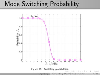
![PA Switching Probability
A switching probability for given target rate R b/s/Hz
fm = Pr(Rm−1 < R ≤ Rm)
= (Υm−1 − Υm) (Υm−1 + Υm − 2)
by using order statistics [David, 1970, Proakis and Salehi, 2007]
- Υm 2R
− 1 σ2
m + 1 e−(2R
−1)σ2
m
- σ2
m
σ2
z
AµmP max
out
, where σ2
z is variance of AWGN
- Υ0 = 0 and ΥM+2 = 1
EE of the proposed TAS-MRC systems for the given R
EETAS
MRC =
ΩR(1 − fM+2)
M+2
m=1 PTx,mfm
- PTx,m
100cµmP max
out
ǫ(µm)
+ Pfix, if m = 1, . . . , M + 1,
Pfix, if m = M + 2 (off-mode)
Jingon Joung Tutorial 2: Energy Efficient Wireless Communications 69 / 112](https://image.slidesharecdn.com/tutorialiceic2015-150603000145-lva1-app6892/85/Energy-Efficient-Wireless-Communications-127-320.jpg)
![PA Switching Probability
A switching probability for given target rate R b/s/Hz
fm = Pr(Rm−1 < R ≤ Rm)
= (Υm−1 − Υm) (Υm−1 + Υm − 2)
by using order statistics [David, 1970, Proakis and Salehi, 2007]
- Υm 2R
− 1 σ2
m + 1 e−(2R
−1)σ2
m
- σ2
m
σ2
z
AµmP max
out
, where σ2
z is variance of AWGN
- Υ0 = 0 and ΥM+2 = 1
EE of the proposed TAS-MRC systems for the given R
EETAS
MRC =
ΩR(1 − fM+2)
M+2
m=1 PTx,mfm
- PTx,m
100cµmP max
out
ǫ(µm)
+ Pfix, if m = 1, . . . , M + 1,
Pfix, if m = M + 2 (off-mode)
Jingon Joung Tutorial 2: Energy Efficient Wireless Communications 69 / 112](https://image.slidesharecdn.com/tutorialiceic2015-150603000145-lva1-app6892/85/Energy-Efficient-Wireless-Communications-128-320.jpg)


![EE Comparison
Simulation
Environments
PA1(0.63 W, 55%),
PA2(2.5 W, 43%),
PA3(10 W, 60%)
8 dB IBO
Switch insertion loss:
GS = 0 dB for S1,
GS = 1 dB for S2
Channel attenuation:
A dB = G − 128 +
10 log10(d−α)
[LTE, 2011]
G = 5 dB,
d = 0.6 km, α = 3.76
σ2 = −174 dBm / Hz,
Ω = 10 MHz,
Pfix = 40 W and
c = 4.7
[Joung et al., 2014c]
0 1 2 3 4 5 6 7 8 9 10 11 12 13 14 15
0
0.2
0.4
0.6
0.8
1.0
1.2
R b/s/Hz
Energyefficiency(EE)Mb/J
no power control
Figure 27: EE comparison.
Jingon Joung Tutorial 2: Energy Efficient Wireless Communications 72 / 112](https://image.slidesharecdn.com/tutorialiceic2015-150603000145-lva1-app6892/85/Energy-Efficient-Wireless-Communications-135-320.jpg)
![EE Comparison
Simulation
Environments
PA1(0.63 W, 55%),
PA2(2.5 W, 43%),
PA3(10 W, 60%)
8 dB IBO
Switch insertion loss:
GS = 0 dB for S1,
GS = 1 dB for S2
Channel attenuation:
A dB = G − 128 +
10 log10(d−α)
[LTE, 2011]
G = 5 dB,
d = 0.6 km, α = 3.76
σ2 = −174 dBm / Hz,
Ω = 10 MHz,
Pfix = 40 W and
c = 4.7
[Joung et al., 2014c]
0 1 2 3 4 5 6 7 8 9 10 11 12 13 14 15
0
0.2
0.4
0.6
0.8
1.0
1.2
R b/s/Hz
Energyefficiency(EE)Mb/J
1-bit FB for off-mode
off-mode
gain
Figure 27: EE comparison.
Jingon Joung Tutorial 2: Energy Efficient Wireless Communications 72 / 112](https://image.slidesharecdn.com/tutorialiceic2015-150603000145-lva1-app6892/85/Energy-Efficient-Wireless-Communications-136-320.jpg)
![EE Comparison
Simulation
Environments
PA1(0.63 W, 55%),
PA2(2.5 W, 43%),
PA3(10 W, 60%)
8 dB IBO
Switch insertion loss:
GS = 0 dB for S1,
GS = 1 dB for S2
Channel attenuation:
A dB = G − 128 +
10 log10(d−α)
[LTE, 2011]
G = 5 dB,
d = 0.6 km, α = 3.76
σ2 = −174 dBm / Hz,
Ω = 10 MHz,
Pfix = 40 W and
c = 4.7
[Joung et al., 2014c]
0 1 2 3 4 5 6 7 8 9 10 11 12 13 14 15
0
0.2
0.4
0.6
0.8
1.0
1.2
R b/s/Hz
Energyefficiency(EE)Mb/J
2-bit FB for Pow Ctrl
off-mode
power
control
gain
gain
Figure 27: EE comparison.
Jingon Joung Tutorial 2: Energy Efficient Wireless Communications 72 / 112](https://image.slidesharecdn.com/tutorialiceic2015-150603000145-lva1-app6892/85/Energy-Efficient-Wireless-Communications-137-320.jpg)
![EE Comparison
Simulation
Environments
PA1(0.63 W, 55%),
PA2(2.5 W, 43%),
PA3(10 W, 60%)
8 dB IBO
Switch insertion loss:
GS = 0 dB for S1,
GS = 1 dB for S2
Channel attenuation:
A dB = G − 128 +
10 log10(d−α)
[LTE, 2011]
G = 5 dB,
d = 0.6 km, α = 3.76
σ2 = −174 dBm / Hz,
Ω = 10 MHz,
Pfix = 40 W and
c = 4.7
[Joung et al., 2014c]
0 1 2 3 4 5 6 7 8 9 10 11 12 13 14 15
0
0.2
0.4
0.6
0.8
1.0
1.2
R b/s/Hz
Energyefficiency(EE)Mb/J
2-bit FB for Pow Ctrl
2-bit FB for PAS
Figure 27: EE comparison.
Jingon Joung Tutorial 2: Energy Efficient Wireless Communications 72 / 112](https://image.slidesharecdn.com/tutorialiceic2015-150603000145-lva1-app6892/85/Energy-Efficient-Wireless-Communications-138-320.jpg)
![MIMO Syst. with Partial CSIT
x2
x1
z2
z1
y2
y1
MRC/MIMO
ˆx2
ˆx1
√
Ah2
√
Ah1
M +1
M +1 Ant.2
Ant.1
: high-power main power amplifiers
PC
PC
power contorl
feedback for PC
Figure 28: PAS MIMO system model with two main PA and M auxiliary PAs.
Switch S0 selects a communication mode
Switch S1 selects a PA [Joung et al., 2014d]
µmPmax
out : Maximum output power of PA m ∈ {1, · · · , M + 1}
0 < µ1 < · · · < µM < µM+1 = 1
2Pmax
out : maximum output power of TX subject to regulatory constraints
Jingon Joung Tutorial 2: Energy Efficient Wireless Communications 73 / 112](https://image.slidesharecdn.com/tutorialiceic2015-150603000145-lva1-app6892/85/Energy-Efficient-Wireless-Communications-139-320.jpg)
![MIMO Syst. with Partial CSIT
x2
x1
z2
z1
y2
y1
MRC/MIMO
ˆx2
ˆx1
√
Ah2
√
Ah1S0
S1
M +1
M +1
M
1
Ant.2
Ant.1
0
0
M + 1
M
1
1
: high-power main power amplifiers
: low-power auxiliary power amplifiers
feedback for S1 and S2
...
off-mode
Figure 28: PAS MIMO system model with two main PA and M auxiliary PAs.
Switch S0 selects a communication mode
Switch S1 selects a PA [Joung et al., 2014d]
µmPmax
out : Maximum output power of PA m ∈ {1, · · · , M + 1}
0 < µ1 < · · · < µM < µM+1 = 1
2Pmax
out : maximum output power of TX subject to regulatory constraints
Jingon Joung Tutorial 2: Energy Efficient Wireless Communications 73 / 112](https://image.slidesharecdn.com/tutorialiceic2015-150603000145-lva1-app6892/85/Energy-Efficient-Wireless-Communications-140-320.jpg)

![EE Analysis
EE can be derived as EEPAS
MIMO = ΩR(1−fM+3)
M+3
m=1
PTx,mfm
.
- Numerator represents system throughput over bandwidth Ω Hz and given
target rate R
- Denominator is total power consumption with model defined as
[Joung et al., 2013, H´eliot et al., 2012]:
PTx,m =
Pant,m + Psp1Ω + Pfix, if m = 1, · · · , M + 1,
2Pant,m + Psp1Ω + Pfix, if m = M + 2,
Pfix, if m = M + 3
+ Pant,m: power consumption that is proportional to the number of transmit
antennas NT [Xu et al., 2011], as Pant,m =
cµmP max
out
ǫ(µm)
+ Pcc + Psp2Ω
+ c: a system dependent power loss coefficient which can be empirically
measured and obtained
+ ǫ(µm): a PA efficiency that depends on the input power (or equivalently PA
output power)
+ Pcc and Psp2 are the RF circuit and signal processing related power
consumptions per bandwidth, respectively, which are proportional to NT
+ µ4 = µ3
+ Psp1: a sig. proc.g related power consumption which is independent of NT
+ Pfix: a fixed power consumption, for power supply and cooling system, which
is independent of P max
out , NT , and Ω
Jingon Joung Tutorial 2: Energy Efficient Wireless Communications 75 / 112](https://image.slidesharecdn.com/tutorialiceic2015-150603000145-lva1-app6892/85/Energy-Efficient-Wireless-Communications-142-320.jpg)


![System Model [Joung et al., 2014a]
BBU
deactivated DA
user equipment
SISO MISO MU-MIMO
activated DA
optical fibre
large-scale
distributed antennas
(DAs)
cellular
communication
networks
Jingon Joung Tutorial 2: Energy Efficient Wireless Communications 80 / 112](https://image.slidesharecdn.com/tutorialiceic2015-150603000145-lva1-app6892/85/Energy-Efficient-Wireless-Communications-149-320.jpg)


![Power Consumption Model: TPI
TPI term
g(S, W ) = grf(S) + gbb(W ) + gnet(M) + Pfix
grf(S) = m∈M
Pcc1,m + Pcc2,m u∈U
Ru maxu smu
gbb(W ) = ΩPsp1 [dim(W )]β+1
+ ΩPsp2
gnet(M) = MΩPsig
Pcc1: eRF
Pcc2: per unit-bit-and-second of oRF
Ru: target rate of user u
β ≥ 0: implies overhead power consumption of MU processing compared to
SU-MIMO
Pfix: fixed power consumption (e.g., pow supply, AC/DC, DC/DC, and
cooling system)
Jingon Joung Tutorial 2: Energy Efficient Wireless Communications 83 / 112](https://image.slidesharecdn.com/tutorialiceic2015-150603000145-lva1-app6892/85/Energy-Efficient-Wireless-Communications-154-320.jpg)
![EE of L-DAS
EE (S, W, P ) =
u∈U
Ω log2 1 +
|hr
u (sc
u ◦ wc
u)|
2
puu
U
u′=1,u′=u |hr
u (sc
u′ ◦ wc
u′ )|2
pu′u′ + σ2
m∈M
c
ηm
(S ◦ W )P (S ◦ W )H
mm
+
m∈M
Pcc1,m + Pcc2,m
u∈U
Ru max
u
smu
+ ΩPsp1 [dim(W )]
β+1
+ ΩPsp2
+ MΩPsig
Jingon Joung Tutorial 2: Energy Efficient Wireless Communications 84 / 112](https://image.slidesharecdn.com/tutorialiceic2015-150603000145-lva1-app6892/85/Energy-Efficient-Wireless-Communications-155-320.jpg)


![ZF-MU-MIMO Precoding Design
Pℓ,1: Precoding matrix W ∗
ℓ for fixed S∗
ℓ and P ′
ℓ
W ∗
ℓ = max
Wℓ
EE(S∗
ℓ , Wℓ, P ′
ℓ )
(a)
≡ min
Wℓ
C(S∗
ℓ , Wℓ, P ′
ℓ )
(b)
≡ min
Wℓ
c
m∈Mℓ
1
ηm
(S∗
ℓ ◦ Wℓ)P ′
ℓ (S∗
ℓ ◦ Wℓ)H
mm
(c)
≡ min
Wℓ
m∈Mℓ
(S∗
ℓ ◦ Wℓ)P ′
ℓ (S∗
ℓ ◦ Wℓ)H
mm
(a) rate does not depend on Wℓ due to a ZF property
(b) Wℓ affects only on TPD term for given S∗
ℓ
and P ′
ℓ
(c) equal capability of PA is preferred for high EE [Joung and Sun, 2013],
c/ηm is assumed to be a constant
Jingon Joung Tutorial 2: Energy Efficient Wireless Communications 92 / 112](https://image.slidesharecdn.com/tutorialiceic2015-150603000145-lva1-app6892/85/Energy-Efficient-Wireless-Communications-181-320.jpg)


![Cont.: Heuristic Method
Minimum required power to satisfy Ru with ZF-MU-MIMO precoding
pu,ℓ = σ2
2
Ru
Ω − 1
pu,ℓ is a ratio based on minimum required power for target rate
[Joung and Sun, 2013] s.t.
pu,ℓ =
pu,ℓ
k∈Uℓ
pk,ℓ
, ∀u ∈ Uℓ
pu,ℓ = αℓpu,ℓ
αℓ: common power scaling factor for power limit of PAs and target rate of
UEs in cluster ℓ
Maximize EE lower bound
Jingon Joung Tutorial 2: Energy Efficient Wireless Communications 95 / 112](https://image.slidesharecdn.com/tutorialiceic2015-150603000145-lva1-app6892/85/Energy-Efficient-Wireless-Communications-186-320.jpg)
![Cont.: Heuristic Method
§
¦
¤
¥
P′
ℓ,2 : α∗
ℓ = arg max
αℓ
ζ(αℓ), s.t. αLB,ℓ ≤ αℓ ≤ αUB,ℓ
ζ(αℓ) =
ΩUℓ log2(1+c1,ℓαℓ)
c2,ℓαℓ+c3,ℓ
: concave function
c1,ℓ minu{pu,ℓ}σ−2
c2,ℓ c m∈Mℓ
η−1
m [Sd
ℓ W ∗
ℓ P ℓ(Sd
ℓ W ∗H
ℓ )H
]mm
c3,ℓ = m∈Mℓ
(Pcc1,m + Pcc2,m u∈Uℓ
Ru) maxu∈Uℓ
smu +
ΩPsp1[dim(Wℓ)]β+1
+ MℓΩPsig + ΩPsp2/L + Pfix/L
αLB,ℓ = σ2
2
Ru
Ω − 1 pu,ℓ from QoS constraint
αUB,ℓ = minm∈Mℓ
Pm Sd
ℓ W ∗
ℓ P ℓ(Sd
ℓ W ∗
ℓ )H
mm
from power constraint
Jingon Joung Tutorial 2: Energy Efficient Wireless Communications 96 / 112](https://image.slidesharecdn.com/tutorialiceic2015-150603000145-lva1-app6892/85/Energy-Efficient-Wireless-Communications-187-320.jpg)
![Cont.: Solution
Closed form solution:
αo =
1
c1
exp 1 + W −
1
exp(1)
+
c1c3
c2exp(1)
− 1
α∗
= [αo]
αUB
αLB
P ∗
heuristic = α∗
P
Jingon Joung Tutorial 2: Energy Efficient Wireless Communications 97 / 112](https://image.slidesharecdn.com/tutorialiceic2015-150603000145-lva1-app6892/85/Energy-Efficient-Wireless-Communications-188-320.jpg)


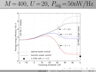


![Envelope Tracking Architecture B
the envelope tracking RF PA’s supply voltage is controlled by the envelope
of the RF-drive.
efficiency between the linear RF PA and the PAs using the Kahn technique.
Figure 31: Envelope tracking architecture [Raab et al., 2003c].
Jingon Joung Tutorial 2: Energy Efficient Wireless Communications 114 / 112](https://image.slidesharecdn.com/tutorialiceic2015-150603000145-lva1-app6892/85/Energy-Efficient-Wireless-Communications-206-320.jpg)
![Doherty Technique B
Class-B (carrier PA or main PA) and class-C (peaking PA or auxiliary PA)
PAs are combined to improve efficiency
The class-B PA is activated if the signal amplitude is half or less than the
PEP
Both PAs are activated if the signal amplitude is larger than half of the
PEP [Doherty, 1936]
Due to the high efficiency and linearity over wide frequency band and
power level, Doherty technique is widely used for the modern cellular
communications [Correia et al., 2010, Cha et al., 2004, Auer et al., 2011,
Arnold et al., 2010].
RF-drive input output
main PA
auxiliary PA
Figure 32: Doherty transmitter.
Jingon Joung Tutorial 2: Energy Efficient Wireless Communications 115 / 112](https://image.slidesharecdn.com/tutorialiceic2015-150603000145-lva1-app6892/85/Energy-Efficient-Wireless-Communications-207-320.jpg)
![Reference I
[McK, 2007] (2007).
The impact of ICT on global emissions.
Technical report, McKinsey & Company.
[Alc, 2008] (2008).
Active antenna arrays: Small-footprint, scalable RF solutions for base stations.
Technical report, Alcatel-Lucent Innovation Days.
[LTE, 2011] (2011).
LTE; E-UTRA; RF requirements for LTE pico node B.
[3GPP, TR 25.927 V11.0.0, 2012] 3GPP, TR 25.927 V11.0.0 (2012).
Solutions for energy saving within UTRA Node B (Release 11).
[Adachi et al., 2012] Adachi, K., Joung, J., Sun, S., and Tan, P. H. (2012).
Energy-saving coordinated napping (CoNap) for wireless networks.
In Proc. IEEE Global Commun. Conf. (GLOBECOM), Anaheim, CA, USA.
[Adachi et al., 2013] Adachi, K., Joung, J., Sun, S., and Tan, P. H. (2013).
Adaptive coordinated napping (CoNap) for energy saving in wireless networks.
IEEE Trans. Wireless Commun., 12(11):5656–5667.
Jingon Joung Tutorial 2: Energy Efficient Wireless Communications 116 / 112](https://image.slidesharecdn.com/tutorialiceic2015-150603000145-lva1-app6892/85/Energy-Efficient-Wireless-Communications-208-320.jpg)
![Reference II
[Arnold et al., 2010] Arnold, O., Richter, F., Fettweis, G., and Blume, O. (2010).
Power consumption modeling of different base station types in heterogeneous cellular
networks.
In Proc. IEEE Future Network and Mobile Summit 2010, Florence, Italy.
[Auer et al., 2011] Auer, G., Giannini, V., Desset, C., G´odor, I., Skillermark, P., Olsson, M.,
Imran, M. A., Sabella, D., Gonzalez, M. J., Blume, O., and Fehske, A. (2011).
How much energy is needed to run a wireless network?
IEEE Trans. Wireless Commun., 18:40–49.
[Baliga et al., 2011] Baliga, J., Ayre, R., Hinton, K., and Tucker, R. S. (2011).
Energy consumption in wired and wireless access networks.
IEEE Commun. Mag., 49:70–77.
[Bogucka and Conti, 2011] Bogucka, H. and Conti, A. (2011).
Degree of freedom for energy savings in practical adaptive wireless systems.
IEEE Commun. Mag., 49:38–45.
Jingon Joung Tutorial 2: Energy Efficient Wireless Communications 117 / 112](https://image.slidesharecdn.com/tutorialiceic2015-150603000145-lva1-app6892/85/Energy-Efficient-Wireless-Communications-209-320.jpg)
![Reference III
[Boumaiza and Ghannouchi, 2003] Boumaiza, S. and Ghannouchi, F. (2003).
Thermal memory effects modeling and compensation in RF power amplifiers and
predistortion linearizers.
IEEE Trans. Microw. Theory Tech., 51:2427–2433.
[Bussgang, 1952] Bussgang, J. J. (1952).
Cross correlation function of amplitude-distorted Gaussian input signals.
Res. Lab Electron., M.I.T., Cambridge, MA, Tech. Rep. 216, 3.
[Cha et al., 2004] Cha, J., Kim, J., Kim, B., Lee, J. S., and Kim, S. H. (2004).
Highly efficient power amplifier for CDMA base stations using Doherty configuration.
In Proc. IEEE MTT-S Int. Microwave Symp., pages 553–556, Fort Worth, TX, USA.
[Chapeau-Blondeau and Monir, 2002] Chapeau-Blondeau, F. and Monir, A. (2002).
Numerical evaluation of the Lambert W function and application to generation of
generalized gaussian noise with exponent 1/2.
IEEE Trans. Signal Process., 50:2160–2165.
[Chatzipapas et al., 2011] Chatzipapas, A., Alouf, S., and Mancuso, V. (2011).
On the minimization of power consumption in base stations using on/off power amplifiers.
In Proc. IEEE Online Conference on Green Communications (GreenCom), pages 18–23.
Jingon Joung Tutorial 2: Energy Efficient Wireless Communications 118 / 112](https://image.slidesharecdn.com/tutorialiceic2015-150603000145-lva1-app6892/85/Energy-Efficient-Wireless-Communications-210-320.jpg)
![Reference IV
[Chen et al., 2011] Chen, Y., Zhang, S., Xu, S., and Li, G. Y. (2011).
Fundamental trade-offs on green wireless networks.
IEEE Commun. Mag., 49:30–37.
[Choi and Andrews, 2007] Choi, W. and Andrews, J. G. (2007).
Downlink performance and capacity of distributed antenna systems in a multicell
environment.
IEEE Trans. Wireless Commun., 6:69–73.
[Correia et al., 2010] Correia, L. M., Zeller, D., Blume, O., Ferling, D., Jading, Y., G´odor, I.,
Auer, G., and der Perre, L. V. (2010).
Challenges and enabling technologies for energy aware mobile radio networks.
IEEE Commun. Mag., 48:66–72.
[Cover and Thomas, 2006] Cover, T. M. and Thomas, J. A. (2006).
Elements of information theory.
John Wiley & Sons, New Jersey, second edition.
[Cox, 1974] Cox, D. (1974).
Linear amplification with nonlinear components.
IEEE Trans. Commun., 22:1942–1945.
Jingon Joung Tutorial 2: Energy Efficient Wireless Communications 119 / 112](https://image.slidesharecdn.com/tutorialiceic2015-150603000145-lva1-app6892/85/Energy-Efficient-Wireless-Communications-211-320.jpg)
![Reference V
[Cripps, 2006] Cripps, S. C. (2006).
RF power amplifiers for wireless communications.
ARTECH HOUSE, Boston/London, second edition.
[Damnjanovic et al., 2011] Damnjanovic, A., Montojo, J., Wei, Y., Ji, T., Luo, T.,
Vajapeyam, M., Yoo, T., Song, O., and Malladi, D. (2011).
A survey on 3GPP heterogeneous networks.
18(3):10–21.
[David, 1970] David, H. A. (1970).
Order staistics.
Wiley, New York,.
[Deruyck et al., 2011] Deruyck, M., Tanghe, E., Joseph, W., and Martens, L. (2011).
Modelling the energy efficiency of microcell base stations.
In Proc. Int. Conf. Smart Grids, Green Commun. and IT Energy-aware Technol., Venice,
Italy.
Jingon Joung Tutorial 2: Energy Efficient Wireless Communications 120 / 112](https://image.slidesharecdn.com/tutorialiceic2015-150603000145-lva1-app6892/85/Energy-Efficient-Wireless-Communications-212-320.jpg)
![Reference VI
[Deruyck et al., 2010] Deruyck, M., Vereecken, W., Tanghe, E., Joseph, W., Pickavet, M.,
Martens, L., and Demeester, P. (2010).
Comparison of power consumption of mobile WiMAX, HSPA and LTE access networks.
In Proc. IEEE Telecommunications Internet and Media Techno Economics (CTTE), Gent,
Belgium.
[Doherty, 1936] Doherty, W. H. (1936).
A new high efficiency power amplifier for modulated waves.
IEEE Proceedings of the Institute of Radio Engineers (IRE), 24:1163–1182.
[earth, 2015] earth (2015).
Energy aware radio and network technology (EARTH) project.
[Falconer et al., 2000] Falconer, D., Kolze, T., Leiba, Y., and Liebetreu, J. (2000).
System impairment model.
[Fettweis and Zimmermann, 2008] Fettweis, G. and Zimmermann, E. (2008).
ICT energy consumption? Trends and challenges.
In Proc. Wireless Personal Multimedia Commun., Lapland, Finland.
Jingon Joung Tutorial 2: Energy Efficient Wireless Communications 121 / 112](https://image.slidesharecdn.com/tutorialiceic2015-150603000145-lva1-app6892/85/Energy-Efficient-Wireless-Communications-213-320.jpg)
![Reference VII
[Frenger et al., 2011] Frenger, P., Moberg, P., Malmodin, J., Jading, Y., and G´odor, I.
(2011).
Reducing energy consumption in LTE with cell DTX.
In Proc. IEEE Veh. Technol. Conf. (VTC-Spring), Budapest, Hungary.
[Gadringer et al., 2005] Gadringer, M., Arthaber, H., Mayer, M., and Magerl, G. (2005).
Modeling, analysis and classification of a PA based on identified Volterra kernels.
In Proc. Gallium Arsenide and Other Semiconductor Application Symposium (GAAS),
pages 405–408, Paris, France.
[Ghorbani and Sheikhan, 1991] Ghorbani, A. and Sheikhan, M. (1991).
The effect of solid state power amplifiers (SSPAs) nonlinearities on MPSK and M-QAM
signal transmission.
In Proc. Inter. Conf. Digital Processing of Signals in Commun., pages 193–197,
Loughborough, UK.
[Gruber et al., 2009] Gruber, M., Blume, O., Ferling, D., Zeller, D., and Imran, M. A. (2009).
EARTH–Energy aware radio and network technologies.
In Proc. IEEE Int. Symp. on Personal, Indoor and Mobile Radio Commun. (PIMRC),
Tokyo, Japan.
Jingon Joung Tutorial 2: Energy Efficient Wireless Communications 122 / 112](https://image.slidesharecdn.com/tutorialiceic2015-150603000145-lva1-app6892/85/Energy-Efficient-Wireless-Communications-214-320.jpg)
![Reference VIII
[Gutman and Wulich, 2012] Gutman, I. and Wulich, D. (2012).
On achievable rate of multicarrier with practical high power amplifier.
In European Wireless 2012 (EW2012), Poznan, Poland.
[Han et al., 2011] Han, S., Yang, C., Wang, G., and Lei, M. (2011).
On the energy efficiency of base station sleeping with multicell cooperative transmission.
In Proc. IEEE Int. Symp. on Personal, Indoor and Mobile Radio Commun. (PIMRC), pages
1536–1540, Toronto, ON, Canada.
[Hasan et al., 2011] Hasan, Z., Boostanimehr, H., and Bhargava, V. K. (2011).
Green cellular networks: A survey, some research issues and challenges.
IEEE Communications Surveys & Tutorials, 13:524–540.
[H´eliot et al., 2012] H´eliot, F., Imran, M. A., and Tafazolli, R. (2012).
On the energy efficiency-spectral efficiency trade-off over the MIMO Rayleigh fading
channel.
IEEE Trans. Commun., pages 1345–1356.
[ITRS, 2011] ITRS (2011).
International technology roadmap for semiconductors.
Jingon Joung Tutorial 2: Energy Efficient Wireless Communications 123 / 112](https://image.slidesharecdn.com/tutorialiceic2015-150603000145-lva1-app6892/85/Energy-Efficient-Wireless-Communications-215-320.jpg)
![Reference IX
[Jeruchim et al., 2000] Jeruchim, M. C., Balaban, P., and Shanmugan, K. S. (2000).
Simulation of communication systems: Modeling, methodology, and techniques.
Springer, New York.
[Jiang and Wu, 2008] Jiang, T. and Wu, Y. (2008).
An overview: Peak-to-average power ratio reduction techniques for OFDM signals.
IEEE Trans. Broadcast., 54:257–268.
[Joung et al., 2014a] Joung, J., Chia, Y. K., and Sun, S. (2014a).
Energy-efficient, large-scale distributed-antenna system (L-DAS) for multiple users.
IEEE J. Sel. Topics Signal Process., 8:954–965.
[Joung et al., 2014b] Joung, J., Ho, C. K., Adachi, K., and Sun, S. (2014b).
A survey on power-amplifier-centric techniques for spectrum and energy efficient wireless
communications.
IEEE Commun., Surveys & Tutorials, pages 1–20.
(early access articles).
Jingon Joung Tutorial 2: Energy Efficient Wireless Communications 124 / 112](https://image.slidesharecdn.com/tutorialiceic2015-150603000145-lva1-app6892/85/Energy-Efficient-Wireless-Communications-216-320.jpg)
![Reference X
[Joung et al., 2012a] Joung, J., Ho, C. K., and Sun, S. (2012a).
Tradeoff of spectral and energy efficiencies: Impact of power amplifier on OFDM systems.
In Proc. IEEE Global Commun. Conf. (GLOBECOM), pages 3274–3279, Anaheim, CA,
USA.
[Joung et al., 2013] Joung, J., Ho, C. K., and Sun, S. (2013).
Power amplifier switching (PAS) for energy efficient systems.
IEEE Wireless Commun. Lett., 2:14–17.
[Joung et al., 2014c] Joung, J., Ho, C. K., and Sun, S. (2014c).
Spectral efficiency and energy efficiency of OFDM systems: Impact of power amplifiers and
countermeasures.
IEEE J. Sel. Areas Commun., 32:208–220.
[Joung et al., 2014d] Joung, J., Ho, C. K., and Sun, S. (2014d).
Tradeoff of spectral and energy efficiencies: Impact of power amplifier on OFDM systems.
In Proc. IEEE Global Commun. Conf. (GLOBECOM), Austin, TX, USA.
Jingon Joung Tutorial 2: Energy Efficient Wireless Communications 125 / 112](https://image.slidesharecdn.com/tutorialiceic2015-150603000145-lva1-app6892/85/Energy-Efficient-Wireless-Communications-217-320.jpg)
![Reference XI
[Joung et al., 2012b] Joung, J., Ho, C. K., Tan, P. H., and Sun, S. (2012b).
Energy minimization in OFDMA downlink systems: A sequential linear assignment
algorithm for resource allocation.
IEEE Wireless Commun. Lett., 1(4):300–303.
[Joung et al., ] Joung, J., Nguyen, H. D., and Sun, S.
Pecuniary efficiency of distributed antenna systems.
1st round revision, Jan. 2015.
[Joung and Sun, 2012] Joung, J. and Sun, S. (2012).
Power efficient resource allocation for downlink OFDMA relay cellular networks.
IEEE Trans. Signal Process., 60:2447–2459.
[Joung and Sun, 2013] Joung, J. and Sun, S. (2013).
Energy efficient power control for distributed transmitters with ZF-based multiuser MIMO
precoding.
IEEE Commun. Lett., 17:1766–1769.
Jingon Joung Tutorial 2: Energy Efficient Wireless Communications 126 / 112](https://image.slidesharecdn.com/tutorialiceic2015-150603000145-lva1-app6892/85/Energy-Efficient-Wireless-Communications-218-320.jpg)
![Reference XII
[Joung et al., 2012c] Joung, J., Yuan, D., Ho, C. K., and Sun, S. (2012c).
Energy efficient network-flow-based algorithm with flow size adaptation for multiuser
multicarrier systems.
IET Networks, 1(2):66–73.
[Kahn, 1952] Kahn, L. (1952).
Single-sideband transmission by envelope elimination and restoration.
IEEE Proceedings of the Institute of Radio Engineers (IRE), 40:803–806.
[Kazimierczuk, 2008] Kazimierczuk, M. K. (2008).
RF power amplifiers.
John Wiley & Sons, UK, first edition.
[Kenington, 2000] Kenington, P. B. (2000).
High linearity RF amplifier design.
Artech House, Norwood, MA.
[Kim and Konstantinou, 2001] Kim, J. and Konstantinou, K. (2001).
Digital predistortion of wideband signals based on power amplifier model with memory.
Electron. Lett., 27:1417–1418.
Jingon Joung Tutorial 2: Energy Efficient Wireless Communications 127 / 112](https://image.slidesharecdn.com/tutorialiceic2015-150603000145-lva1-app6892/85/Energy-Efficient-Wireless-Communications-219-320.jpg)
![Reference XIII
[Kosta et al., 2013] Kosta, C., Quddus, B. H. A., and Tafazolli, R. (2013).
On interference avoidance through inter-cell interference coordination (ICIC) based on
OFDMA mobile systems.
IEEE Commun. Surveys Tuts., 15(3):973–995.
[Kowlgi and Berland, 2011] Kowlgi, S. and Berland, C. (2011).
Linearity considerations for multi-standard cellular base station transmitters.
In Proc. IEEE Microwave Conf. (EuMC), pages 226–229, Manchester, UK.
[Kumar and Gurugubelli, 2011] Kumar, R. V. R. and Gurugubelli, J. (2011).
How green the LTE technology can be?
In Proc. IEEE Wireless Communication, Vehicular Technology, Information Theory and
Aerospace & Electronic Systems Technology (Wireless VITAE), Chennai, India.
[Mancuso and Sara Alouf, 2011] Mancuso, V. and Sara Alouf, I. S. A. M. (2011).
Reducing costs and pollution in cellular networks.
IEEE Wireless Commun. Mag., 17:63–71.
[Minkoff, 1985] Minkoff, J. (1985).
The role of AM-to-PM conversion in memoryless nonlinear systems.
IEEE Trans. Commun., 33(2):139–144.
Jingon Joung Tutorial 2: Energy Efficient Wireless Communications 128 / 112](https://image.slidesharecdn.com/tutorialiceic2015-150603000145-lva1-app6892/85/Energy-Efficient-Wireless-Communications-220-320.jpg)
![Reference XIV
[Morgan et al., 2006] Morgan, D. R., Ma, Z., Kim, J., Zierdt, M. G., and Pastalan, J. (2006).
A generalized memory polynomial model for digital predistortion of RF power amplifiers.
IEEE Trans. Signal Process., 54:3852–3860.
[Niu et al., 2010] Niu, Z., Wu, Y., Gong, J., and Yang, Z. (2010).
Cell zooming for cost-efficient green cellular networks.
IEEE Commun. Mag., 48:74–79.
[Onireti et al., 2012] Onireti, O., H´eliot, F., and Imran, M. A. (2012).
On the energy efficiency-spectral efficiency trade-off in the uplink of CoMP system.
IEEE Trans. Wireless Commun., pages 556–561.
[Papoulis and Pillai, 2002] Papoulis, A. and Pillai, S. (2002).
Probability, random variables and stochastic processes.
McGraw-Hill, fourth edition.
[Pothecary, 1999] Pothecary, N. (1999).
Feedforward Linear Power Amplifiers.
Artech House, Norwood, MA.
Jingon Joung Tutorial 2: Energy Efficient Wireless Communications 129 / 112](https://image.slidesharecdn.com/tutorialiceic2015-150603000145-lva1-app6892/85/Energy-Efficient-Wireless-Communications-221-320.jpg)
![Reference XV
[Proakis and Salehi, 2007] Proakis, J. G. and Salehi, M. (2007).
Digital communications.
McGraw-Hill, New York„ five edition.
[Raab, 1987] Raab, F. H. (1987).
Efficiency of Doherty RF power-amplifier systems.
IEEE Trans. Broadcast., BC-33:77–83.
[Raab et al., 2002] Raab, F. H., Asbeck, P., Cripps, S. C., Kenington, P. B., Popovi´c, Z. B.,
Pothecary, N., Sevic, J. F., and Sokal, N. O. (2002).
Power amplifiers and transmitters for RF and microwave.
IEEE Trans. Microw. Theory Tech., 50:814–826.
[Raab et al., 2003a] Raab, F. H., Asbeck, P., Cripps, S. C., Kenington, P. B., Popovi´c, Z. B.,
Pothecary, N., Sevic, J. F., and Sokal, N. O. (2003a).
RF and microwave power amplifier and transmitter technologies–Part 1.
High Frequency Electronics, pages 22–36.
Jingon Joung Tutorial 2: Energy Efficient Wireless Communications 130 / 112](https://image.slidesharecdn.com/tutorialiceic2015-150603000145-lva1-app6892/85/Energy-Efficient-Wireless-Communications-222-320.jpg)
![Reference XVI
[Raab et al., 2003b] Raab, F. H., Asbeck, P., Cripps, S. C., Kenington, P. B., Popovi´c, Z. B.,
Pothecary, N., Sevic, J. F., and Sokal, N. O. (2003b).
RF and microwave power amplifier and transmitter technologies–Part 2.
High Frequency Electronics, pages 22–36.
[Raab et al., 2003c] Raab, F. H., Asbeck, P., Cripps, S. C., Kenington, P. B., Popovi´c, Z. B.,
Pothecary, N., Sevic, J. F., and Sokal, N. O. (2003c).
RF and microwave power amplifier and transmitter technologies–Part 3.
High Frequency Electronics, pages 34–48.
[Rahmatallah and Mohan, 2013] Rahmatallah, Y. and Mohan, S. (2013).
Peak-to-average power ratio reduction in OFDM systems: A survey and taxonomy.
IEEE Commun. Surveys Tuts., 15(4):1567–1592.
[Rapp, 1991] Rapp, C. (1991).
Effects of HPA-nonlinearity on a 4-DPS/OFDM signal for a digital sound broadcasting
system.
In Proc. Second European Conf. on Satellite Commun., pages 179–184, Lihge, Belgium.
Jingon Joung Tutorial 2: Energy Efficient Wireless Communications 131 / 112](https://image.slidesharecdn.com/tutorialiceic2015-150603000145-lva1-app6892/85/Energy-Efficient-Wireless-Communications-223-320.jpg)
![Reference XVII
[Richter et al., 2009] Richter, F., Fehske, A. J., and Fettweis, G. P. (2009).
Energy efficiency aspects of base station deployment strategies for cellular networks.
In Proc. IEEE Veh. Technol. Conf. (VTC-Fall), Anchorage, AK, USA.
[Saleh, 1981] Saleh, A. A. M. (1981).
Frequency-independent and frequency-dependent nonlinear models of TWT amplifiers.
IEEE Trans. Commun., 29:1715–1720.
[Shirvani et al., 2002] Shirvani, A., Su, D. K., and Wooley, B. A. (2002).
A CMOS RF power amplifier with parallel amplification for efficient power control.
IEEE J. Solid-State Circuits, 27:684–693.
[Staudinger, 2000] Staudinger, J. (2000).
Applying switched gain stage concepts to improve efficiency and linearity for mobile CDMA
power amplification.
Microwave Journal, 43:152–162.
[Teikari, 2008] Teikari, I. (2008).
Digital Predistortion Linearization Methods for RF Power Amplifiers.
PhD thesis, Helsinki University of Technology, Finland.
Jingon Joung Tutorial 2: Energy Efficient Wireless Communications 132 / 112](https://image.slidesharecdn.com/tutorialiceic2015-150603000145-lva1-app6892/85/Energy-Efficient-Wireless-Communications-224-320.jpg)
![Reference XVIII
[Tellado et al., 2003] Tellado, J., Hoo, L. M. C., and Cioffi, J. M. (2003).
Maximum-likelihood detection of nonlinearly distorted multicarrier symbols by iterative
decoding.
IEEE Trans. Commun., 51:218–228.
[Tombaz et al., 2011] Tombaz, S., V¨astberg, A., and Zander, J. (2011).
Energy- and cost-efficient ultra-high-capacity wireless access.
IEEE Trans. Wireless Commun., 18:18–24.
[Verd´u, 2002] Verd´u, S. (2002).
Spectral efficiency in the wideband regime.
IEEE Trans. Inf. Theory, 48(6):1319–1343.
[Vereecken et al., 2011] Vereecken, W., Heddeghem, W. V., Deruyck, M., Puype, B., Lannoo,
B., Joseph, W., Colle, D., Martens, L., and Demeester, P. (2011).
Power consumption in telecommunication networks: overview and reduction strategies.
IEEE Commun. Mag., 49:62–69.
[Vuolevi et al., 2000] Vuolevi, J., Rahkonen, T., and Manninen, J. (2000).
Measurement technique for characterizing memory effects in RF power amplifiers.
In Proc. IEEE Radio and Wireless Conf. (RAWCON), pages 195–198, Denver, CO, USA.
Jingon Joung Tutorial 2: Energy Efficient Wireless Communications 133 / 112](https://image.slidesharecdn.com/tutorialiceic2015-150603000145-lva1-app6892/85/Energy-Efficient-Wireless-Communications-225-320.jpg)
![Reference XIX
[Xu et al., 2011] Xu, J., Qiu, L., and Yu, C. (2011).
Improving energy efficiency through multimode transmission in the downlink MIMO
systems.
EURASIP J. Wireless Commun. Netw., 2011:1–12.
[Yang et al., 2009] Yang, Y., Hu, H., Xu, J., and Mao, G. (2009).
Relay technologies for WiMax and LTE-advanced mobile systems.
IEEE Commun. Mag., 47(10):100–105.
[Zhou et al., 2013] Zhou, L., Hu, R. Q., Qian, Y., and Chen, H.-H. (2013).
Energy-spectrum efficiency tradeoff for video streaming over mobile Ad Hoc networks.
IEEE J. Sel. Areas Commun., 31(5):981–991.
[Zillmann and Fettweis, 2005] Zillmann, P. and Fettweis, G. (2005).
On the capacity of multicarrier transmission over nonlinear channels.
In Proc. IEEE Veh. Technol. Conf. (VTC-Spring), Stockholm, Sweden.
Jingon Joung Tutorial 2: Energy Efficient Wireless Communications 134 / 112](https://image.slidesharecdn.com/tutorialiceic2015-150603000145-lva1-app6892/85/Energy-Efficient-Wireless-Communications-226-320.jpg)

The document discusses energy-efficient wireless communications, focusing on the theoretical and practical tradeoffs between spectral efficiency (SE) and energy efficiency (EE) in various communication technologies. It highlights the significant energy consumption in wireless networks and explores strategies at the device, system, and network levels to improve energy efficiency. The tutorial includes a review of techniques such as power amplifier (PA) switching and large-scale distributed-antenna systems.


![Lecture 1_ EE 406 Introduction to Wireless Networking [Autosaved].pdf](https://cdn.slidesharecdn.com/ss_thumbnails/lecture1ee406introductiontowirelessnetworkingautosaved-241212145646-3509c00d-thumbnail.jpg?width=640&height=640&fit=bounds)


