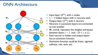
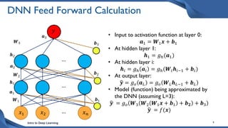
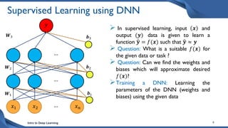
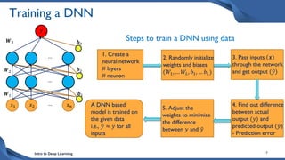
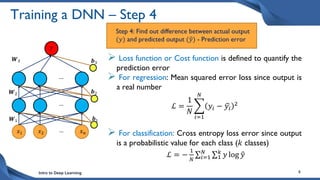
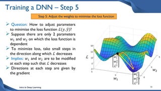
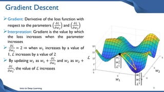
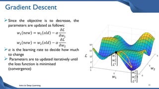
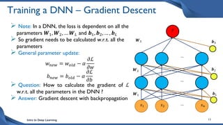
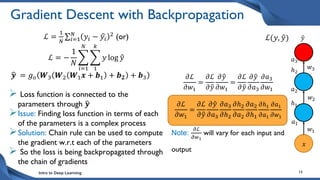
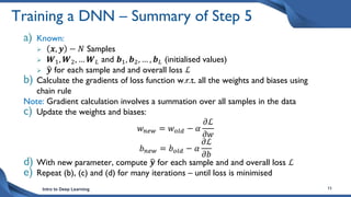
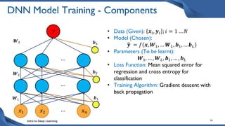
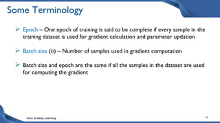
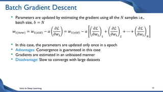
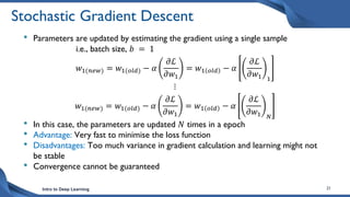
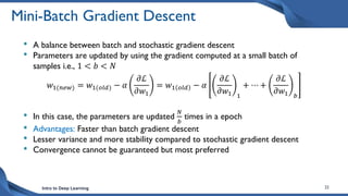
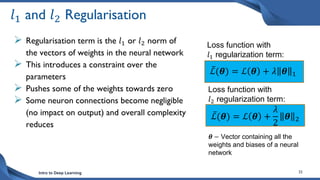
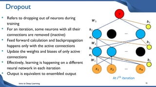
Training DNN Models
Intro to Deep Learning 2
Contents
 Recap of Deep Neural Network
 Training a DNN
 Gradient Descent with Backpropagation
 Variants of Gradient Descent
 Batch Normalisation
 Regularisation
Intro to Deep Learning 3
DNN Architecture
𝑥1 𝑥𝑛
𝑥2 …
…
…
𝑾1 𝒃1
𝑾2 𝒃2
𝑾3 𝒃3
• Input layer (0𝑡ℎ
) with 𝑛 nodes
• 𝐿 − 1 hidden layers with 𝑚 neurons each
• Output layer (𝐿𝑡ℎ
) with 𝑘 neurons
• Neurons in successive layers are connected
to one another
• 𝑾𝑖 and 𝒃𝑖 represent the weights and biases
between layers 𝑖 − 1 and 𝑖 (0 < 𝑖 ≤ 𝐿)
• Each neuron in hidden and output layers
has an activation function
• Activation function could be linear, sigmoid,
softmax, relu, tanh, etc.
𝑦
Intro to Deep Learning 4
DNN Feed Forward Calculation
𝑥1 𝑥𝑛
𝑥2 …
…
…
𝑾1 𝒃1
𝑾2
𝒃2
𝑾3 𝒃3
• Input to activation function at layer 0:
𝒂1 = 𝑾1𝒙 + 𝒃1
• At hidden layer 1:
𝒉1 = 𝑔ℎ(𝒂1)
• At hidden layer i:
𝒉𝑖 = 𝑔ℎ 𝒂𝑖 = 𝑔ℎ(𝑾𝑖𝒉𝑖−1 + 𝒃𝑖)
• At output layer:
𝒚 = 𝑔𝑜 𝒂𝐿 = 𝑔𝑜 𝑾𝐿𝒉𝐿−1 + 𝒃𝐿
• Model (function) being approximated by
the DNN (assuming L=3):
𝒚 = 𝑔𝑜 𝑾3 𝑾2 𝑾1𝒙 + 𝒃1 + 𝒃𝟐 + 𝒃3
𝒚 = 𝑓(𝒙)
𝑦
𝒉2
𝒂2
𝒂1
𝒉1
𝒂3
Intro to Deep Learning 5
Which Activation Function to Use?
 In the 90s, sigmoid and tanh were most popular activation functions
used in neural networks
 Tanh results in faster convergence compared to sigmoid due to zero
centering and larger derivatives
 However, they suffer from vanishing gradient problem as a network
goes deeper
 Therefore, Relu become very popular and default choice for most
neural networks
 However, in RNNs and LSTMs (a variant of neural networks for
handling sequential data), tanh or sigmoid is preferred
Intro to Deep Learning 6
𝑥1 𝑥𝑛
𝑥2 …
…
…
𝑾1 𝒃1
𝑾2 𝒃2
𝑾3 𝒃3
𝑦
Supervised Learning using DNN
 In supervised learning, input 𝒙 and
output (𝒚) data is given to learn a
function 𝒚 = 𝑓(𝒙) such that 𝒚 ≈ 𝒚
 Question: What is a suitable 𝑓(𝒙) for
the given data or task ?
 Question: Can we find the weights and
biases which will approximate desired
𝑓(𝒙)?
Training a DNN: Learning the
parameters of the DNN (weights and
biases) using the given data
Intro to Deep Learning 7
Training a DNN
Steps to train a DNN using data
1. Create a
neural network
# layers
# neuron
2. Randomly initialize
weights and biases
(𝑊1, … 𝑊𝐿, 𝑏1, … 𝑏𝐿)
𝑥1 𝑥𝑛
𝑥2 …
…
…
𝑾1 𝒃1
𝑾2 𝒃2
𝑾3 𝒃3
𝑦
3. Pass inputs 𝒙
through the network
and get output (𝑦)
4. Find out difference
between actual
output (𝑦) and
predicted output (𝑦)
- Prediction error
5. Adjust the
weights to minimise
the difference
between 𝑦 and 𝑦
A DNN based
model is trained on
the given data
i.e., 𝑦 ≈ 𝑦 for all
inputs
Intro to Deep Learning 8
Training a DNN – Step 4
𝑥1 𝑥𝑛
𝑥2 …
…
…
𝑾1 𝒃1
𝑾2 𝒃2
𝑾3 𝒃3
𝑦
Step 4: Find out difference between actual output
(𝑦) and predicted output (𝑦) - Prediction error
 Loss function or Cost function is defined to quantify the
prediction error
 For regression: Mean squared error loss since output is
a real number
ℒ =
1
𝑁
𝑖=1
𝑁
𝑦𝑖 − 𝑦𝑖
2
 For classification: Cross entropy loss error since output
is a probabilistic value for each class (𝑘 classes)
ℒ = −
1
𝑁 𝑖=1
𝑁
1
𝑘
𝑦 log 𝑦
Intro to Deep Learning 10
Training a DNN – Step 5
Step 5: Adjust the weights to minimise the loss function
 Question: How to adjust parameters
to minimise the loss function ℒ(𝑦, 𝑦)?
 Suppose there are only 2 parameters
𝑤1 and 𝑤2 on which the loss function is
dependent
 To minimize loss, take small steps in
the direction along which ℒ decreases
 Implies: 𝑤1 and 𝑤2 are to be modified
at each step such that ℒ decreases
 Directions at each step are given by
the gradient
𝑤1
𝑤1
1
𝑤2
1
ℒ1
𝑤2
ℒ
𝑤1
2
𝑤2
2
ℒ2
Intro to Deep Learning 11
Gradient Descent
Gradient: Derivative of the loss function with
respect to the parameters
𝜕ℒ
𝜕𝑤1
and
𝜕ℒ
𝜕𝑤2
Interpretation: Gradient is the value by which
the loss increases when the parameter
increases
 𝜕ℒ
𝜕𝑤1
= 2 ⇒ when 𝑤1 increases by a value of
1, ℒ increases by a value of 2
 By updating 𝑤1 as 𝑤1 +
𝜕ℒ
𝜕𝑤1
and 𝑤2 as 𝑤2 +
𝜕ℒ
𝜕𝑤2
, the value of ℒ increases
𝑤1
𝑤1
1
𝑤2
1
ℒ1
𝑤2
ℒ
𝑤1
2
𝑤2
2
ℒ2
Intro to Deep Learning 12
Gradient Descent
Since the objective is to decrease, the
parameters are updated as follows:
𝑤1 𝑛𝑒𝑤 = 𝑤1 𝑜𝑙𝑑 − 𝛼
𝜕ℒ
𝜕𝑤1
𝑤2 𝑛𝑒𝑤 = 𝑤2 𝑜𝑙𝑑 − 𝛼
𝜕ℒ
𝜕𝑤2
𝛼 is the learning rate to decide how much
to change
 Parameters are to updated iteratively until
the loss function is minimised
(convergence)
𝑤1
𝑤1
1
𝑤2
1
ℒ1
𝑤2
ℒ
𝑤1
2
𝑤2
2
ℒ2
Intro to Deep Learning 13
Training a DNN – Gradient Descent
 Note: In a DNN, the loss is dependent on all the
parameters 𝑾1, 𝑾2, … 𝑾𝐿 and 𝒃1, 𝒃2, … , 𝒃𝐿
 So gradient needs to be calculated w.r.t. all the
parameters
 General parameter update:
𝑤𝑛𝑒𝑤 = 𝑤𝑜𝑙𝑑 − 𝛼
𝜕ℒ
𝜕𝑤
𝑏𝑛𝑒𝑤 = 𝑏𝑜𝑙𝑑 − 𝛼
𝜕ℒ
𝜕𝑏
 Question: How to calculate the gradient of ℒ
w.r.t. all the parameters in the DNN ?
 Answer: Gradient descent with backpropagation
𝑥1 𝑥𝑛
𝑥2
…
…
…
𝑾1 𝒃1
𝑾2 𝒃2
𝑾3 𝒃3
𝑦
Intro to Deep Learning 14
Gradient Descent with Backpropagation
ℒ =
1
𝑁 𝑖=1
𝑁
𝑦𝑖 − 𝑦𝑖
2 (or)
ℒ = −
1
𝑁
𝑖=1
𝑁
1
𝑘
𝑦 log 𝑦
𝒚 = 𝑔𝑜 𝑾3 𝑾2 𝑾1𝒙 + 𝒃1 + 𝒃𝟐 + 𝒃3
 Loss function is connected to the
parameters through 𝒚
Issue: Finding loss function in terms of each
of the parameters is a complex process
Solution: Chain rule can be used to compute
the gradient w.r.t each of the parameters
 So the loss is being backpropagated through
the chain of gradients
𝑥
𝑤1
𝑎1
ℎ1
𝑤2
𝑤3
ℎ2
𝑎2
𝑎3
𝑦
ℒ(𝑦, 𝑦)
𝜕ℒ
𝜕𝑤1
=
𝜕ℒ
𝜕𝑦
𝜕𝑦
𝜕𝑤1
=
𝜕ℒ
𝜕𝑦
𝜕𝑦
𝜕𝑎3
𝜕𝑎3
𝜕𝑤1
𝜕ℒ
𝜕𝑤1
=
𝜕ℒ
𝜕𝑦
𝜕𝑦
𝜕𝑎3
𝜕𝑎3
𝜕ℎ2
𝜕ℎ2
𝜕𝑎2
𝜕𝑎2
𝜕ℎ1
𝜕ℎ1
𝜕𝑎1
𝜕𝑎1
𝜕𝑤1
Note:
𝜕ℒ
𝜕𝑤1
will vary for each input and
output
Intro to Deep Learning 15
Training a DNN – Summary of Step 5
a) Known:
 𝒙, 𝒚 − 𝑁 Samples
 𝑾1, 𝑾2, … 𝑾𝐿 and 𝒃1, 𝒃2, … , 𝒃𝐿 (initialised values)
 𝒚 for each sample and and overall loss ℒ
b) Calculate the gradients of loss function w.r.t. all the weights and biases using
chain rule
Note: Gradient calculation involves a summation over all samples in the data
c) Update the weights and biases:
𝑤𝑛𝑒𝑤 = 𝑤𝑜𝑙𝑑 − 𝛼
𝜕ℒ
𝜕𝑤
𝑏𝑛𝑒𝑤 = 𝑏𝑜𝑙𝑑 − 𝛼
𝜕ℒ
𝜕𝑏
d) With new parameter, compute 𝒚 for each sample and and overall loss ℒ
e) Repeat (b), (c) and (d) for many iterations – until loss is minimised
Intro to Deep Learning 16
DNN Model Training - Components
• Data (Given): 𝒙𝑖, 𝒚𝑖 ; 𝑖 = 1 … 𝑁
• Model (Chosen):
𝒚 = 𝑓 𝒙, 𝑾1, … 𝑾𝐿, 𝒃1, … 𝒃𝐿
• Parameters (To be learnt):
𝑾1, … , 𝑾𝐿, 𝒃1, … , 𝒃𝐿
• Loss Function: Mean squared error for
regression and cross entropy for
classification
• Training Algorithm: Gradient descent with
back propagation
𝑥1 𝑥𝑛
𝑥2 …
…
…
𝑾1 𝒃1
𝑾2
𝒃2
𝑾3 𝒃3
𝑦
Intro to Deep Learning 17
Variants of Gradient Descent
Intro to Deep Learning 18
Types of Gradient Descent
 Depending on the number of samples used to estimate the gradient of loss
w.r.t. the parameters, there are 3 types of gradient descent:
 Batch Gradient Descent
 Stochastic Gradient Descent
 Mini-Batch Gradient Descent
 Reasons for these 3 types of gradient descent:
 Computational efficiency
 Accuracy of estimated gradient
Intro to Deep Learning 19
Some Terminology
 Epoch – One epoch of training is said to be complete if every sample in the
training dataset is used for gradient calculation and parameter updation
 Batch size (𝑏) – Number of samples used in gradient computation
 Batch size and epoch are the same if all the samples in the dataset are used
for computing the gradient
Intro to Deep Learning 20
Batch Gradient Descent
• Parameters are updated by estimating the gradient using all the 𝑁 samples i.e.,
batch size, 𝑏 = 𝑁
𝑤1(𝑛𝑒𝑤) = 𝑤1(𝑜𝑙𝑑) − 𝛼
𝜕ℒ
𝜕𝑤1
= 𝑤1 𝑜𝑙𝑑 − 𝛼
𝜕ℒ
𝜕𝑤1 1
+
𝜕ℒ
𝜕𝑤1 2
+ ⋯ +
𝜕ℒ
𝜕𝑤1 𝑁
• In this case, the parameters are updated only once in a epoch
• Advantages: Convergence is guaranteed in this case
• Gradients are estimated in an unbisased manner
• Disadvantage: Slow to converge with large datasets
Intro to Deep Learning 21
Stochastic Gradient Descent
• Parameters are updated by estimating the gradient using a single sample
i.e., batch size, 𝑏 = 1
𝑤1(𝑛𝑒𝑤) = 𝑤1(𝑜𝑙𝑑) − 𝛼
𝜕ℒ
𝜕𝑤1
= 𝑤1 𝑜𝑙𝑑 − 𝛼
𝜕ℒ
𝜕𝑤1 1
⋮
𝑤1(𝑛𝑒𝑤) = 𝑤1(𝑜𝑙𝑑) − 𝛼
𝜕ℒ
𝜕𝑤1
= 𝑤1 𝑜𝑙𝑑 − 𝛼
𝜕ℒ
𝜕𝑤1 𝑁
• In this case, the parameters are updated 𝑁 times in a epoch
• Advantage: Very fast to minimise the loss function
• Disadvantages: Too much variance in gradient calculation and learning might not
be stable
• Convergence cannot be guaranteed
Intro to Deep Learning 22
Mini-Batch Gradient Descent
• A balance between batch and stochastic gradient descent
• Parameters are updated by using the gradient computed at a small batch of
samples i.e., 1 < 𝑏 < 𝑁
𝑤1(𝑛𝑒𝑤) = 𝑤1(𝑜𝑙𝑑) − 𝛼
𝜕ℒ
𝜕𝑤1
= 𝑤1 𝑜𝑙𝑑 − 𝛼
𝜕ℒ
𝜕𝑤1 1
+ ⋯ +
𝜕ℒ
𝜕𝑤1 𝑏
• In this case, the parameters are updated
𝑁
𝑏
times in a epoch
• Advantages: Faster than batch gradient descent
• Lesser variance and more stability compared to stochastic gradient descent
• Convergence cannot be guaranteed but most preferred
Intro to Deep Learning 23
Variants of Gradient Descent - Visualisation
Batch Gradient descent
Mini-Batch Gradient descent
Stochastic Gradient descent
• Ellipse with higher radius indicates higher
loss function
Image Source: medium.com
Intro to Deep Learning 24
Batch Normalisation
Intro to Deep Learning 25
Why Batch Normalisation?
• Intuition: All the samples can be
considered to be drawn from a
multi-variate distribution
• If batch gradient descent is
performed, then the distribution of
samples for each batch of inputs
remains the same
• Issue: However, with stochastic and
mini-batch gradient descent, the
distribution varies from one batch to
another.
𝑥1 𝑥𝑛
𝑥2 …
…
…
𝑾1 𝒃1
𝑾2
𝒃2
𝑾3 𝒃3
𝑦
𝒉2
𝒂2
𝒂1
𝒉1
Intro to Deep Learning 26
Why Batch Normalisation?
• Illustration: Suppose the input
samples (𝒙) are fed to the DNN in
multiple mini-batches
• In each iteration, the samples change
and the distribution of samples also
changes
• Weights and biases would have to
adjust to a different distribution of
inputs in each iteration
• Learning (fitting of weights and biases
to inputs) would be hard
• How to overcome this issue? – Batch
Normalisation
𝑥1 𝑥𝑛
𝑥2 …
…
…
𝑾1 𝒃1
𝑾2
𝒃2
𝑾3 𝒃3
𝑦
𝒉2
𝒂2
𝒂1
𝒉1
Intro to Deep Learning 27
Applying Batch Normalisation
• Inputs to each layer are normalised
to be unit gaussians before the
activation function
• Mean and variance across set of
samples in that batch, are calculated
for performing normalisation
• This normalisation step is
differentiable and hence we can
backpropagate through it
• Advantage: Learning is much faster
and leads to be better convergence
𝑥1 𝑥𝑛
𝑥2 …
…
…
𝑾1 𝒃1
𝑾2
𝒃2
𝑾3 𝒃3
𝑦
𝒉2
𝒂2
𝒂1
𝒉1
Ref: Article by Johann Huber - Batch normalization in 3 levels of understanding
Intro to Deep Learning 28
Regularisation
Intro to Deep Learning 29
Regularisation – Motivation
DNN Model Training Objectives:
• Finding a model which is a good fit to the
given data
• Model should be able to generalise over
unseen data (Test data)
• Prediction error should be low both on
training and test data
Issues:
• In DNNs, there is the issue of overfitting due
to many parameters
• Test error could be high due to overfitting
Solution:
• To obtain a balanced model, regularisation is
performed
Model complexity
Error
Test
error
Train
error
Ideal model
complexity
Intro to Deep Learning 30
Finding Ideal Model Complexity
• To get near ideal model complexity, an
additional component is added to the loss
function
ℒ 𝜃 + 𝜆Ω(𝜃)
• Ω(𝜃) is the regularisation term which
regularises the model
• Ω(𝜃) ensures that the model is neither too
complex models nor too simple models
• 𝜆 is the regularisation rate (hyperparamter)
• 𝜆 determines how much the model is to be
regularised
Model complexity
Error
Test
error
Train
error
Ideal model
complexity
Intro to Deep Learning 31
Types of Regularization
 𝑙1 and 𝑙2 regularization
 Early stopping
 Ensemble Methods
 Dropout
Intro to Deep Learning 32
𝑙1 and 𝑙2 Regularisation
 Regularisation term is the 𝑙1 or 𝑙2 norm of
the vectors of weights in the neural network
 This introduces a constraint over the
parameters
 Pushes some of the weights towards zero
 Some neuron connections become negligible
(no impact on output) and overall complexity
reduces
ℒ(𝜽) = ℒ 𝜽 +
𝜆
2
𝜽 2
ℒ(𝜽) = ℒ 𝜽 + 𝜆 𝜽 1
Loss function with
𝑙1 regularization term:
Loss function with
𝑙2 regularization term:
𝜽 − Vector containing all the
weights and biases of a neural
network
Intro to Deep Learning 33
Early Stopping
• Prediction error on a validation set is
tracked
• New hyperparameter called patience
parameter 𝑝 is introduced
• Check if there is improvement in the
validation error for 𝑝 continuous
iterations
• If not stop and take the model prior to
those 𝑝 iterations
Error
Validation
error
Train
error
𝑘 − 𝑝
iteration
𝑘𝑡ℎ
iteration
Intro to Deep Learning 34
Ensemble Methods
• Different models are trained for the
same task using different features,
hyperparameters, samples, etc.
• Outputs of these models are
combined to reduce the prediction
error
• Similar to random forest or bagging
of trees
• Computationally very expensive and
hence not preferred
𝑥1 𝑥𝑖
𝑥2 …
…
…
𝑾1 𝒃1
𝑾2 𝒃2
𝑾3 𝒃3
𝑦1
𝑥1 𝑥𝑗
𝑥2 …
…
…
𝑾1 𝒃1
𝑾2 𝒃2
𝑾3 𝒃3
𝑦2
𝑦 =
𝑦1 + 𝑦2
2
Ensemble of 2 DNN models
Intro to Deep Learning 35
Dropout
𝑥1 𝑥𝑛
𝑥2 …
…
…
𝑾1 𝒃1
𝑾2
𝒃2
𝑾3 𝒃3
𝑦
𝒉2
𝒂2
𝒂1
𝒉1
• Refers to dropping out of neurons during
training
• For an iteration, some neurons with all
their connections are removed (inactive)
Intro to Deep Learning 36
Dropout
• Refers to dropping out of neurons during
training
• For an iteration, some neurons with all their
connections are removed (inactive)
• Feed forward calculation and backpropagation
happens only with the active connections
• Update the weights and biases of only active
connections
• Effectively, learning is happening on a different
neural network in each iteration
• Output is equivalent to ensembled output
𝑥1 𝑥𝑛
𝑥2 …
…
…
𝑾1 𝒃1
𝑾2
𝒃2
𝑾3 𝒃3
𝑦
𝒉2
𝒂2
𝒂1
𝒉1
At 𝑖𝑡ℎ iteration
Intro to Deep Learning 37
DNN Training - Demonstration
• https://playground.tensorflow.org/
Intro to Deep Learning 38
Summary
 Training a DNN implies learning the parameters of the neural network
(weights and biases) for modelling a particular function (input-output
relation)
 Training is performed by adjusting the parameters such that the loss
between actual and predicted outputs is minimised
 Loss is backpropagated through the layers of the neural network
following a direction of gradient descent
 Different types of gradient descent approaches have been proposed to
balance between computational efficiency and accuracy of gradients
estimated
 Batch Normalisation is performed to ensure stable learning of parameters
 To avoid overfitting of DNN models, regularisation is performed during
training of DNN models
THANK YOU

Training DNN Models - II.pptx

  • 1.
  • 2.
    Intro to DeepLearning 2 Contents  Recap of Deep Neural Network  Training a DNN  Gradient Descent with Backpropagation  Variants of Gradient Descent  Batch Normalisation  Regularisation
  • 3.
    Intro to DeepLearning 3 DNN Architecture 𝑥1 𝑥𝑛 𝑥2 … … … 𝑾1 𝒃1 𝑾2 𝒃2 𝑾3 𝒃3 • Input layer (0𝑡ℎ ) with 𝑛 nodes • 𝐿 − 1 hidden layers with 𝑚 neurons each • Output layer (𝐿𝑡ℎ ) with 𝑘 neurons • Neurons in successive layers are connected to one another • 𝑾𝑖 and 𝒃𝑖 represent the weights and biases between layers 𝑖 − 1 and 𝑖 (0 < 𝑖 ≤ 𝐿) • Each neuron in hidden and output layers has an activation function • Activation function could be linear, sigmoid, softmax, relu, tanh, etc. 𝑦
  • 4.
    Intro to DeepLearning 4 DNN Feed Forward Calculation 𝑥1 𝑥𝑛 𝑥2 … … … 𝑾1 𝒃1 𝑾2 𝒃2 𝑾3 𝒃3 • Input to activation function at layer 0: 𝒂1 = 𝑾1𝒙 + 𝒃1 • At hidden layer 1: 𝒉1 = 𝑔ℎ(𝒂1) • At hidden layer i: 𝒉𝑖 = 𝑔ℎ 𝒂𝑖 = 𝑔ℎ(𝑾𝑖𝒉𝑖−1 + 𝒃𝑖) • At output layer: 𝒚 = 𝑔𝑜 𝒂𝐿 = 𝑔𝑜 𝑾𝐿𝒉𝐿−1 + 𝒃𝐿 • Model (function) being approximated by the DNN (assuming L=3): 𝒚 = 𝑔𝑜 𝑾3 𝑾2 𝑾1𝒙 + 𝒃1 + 𝒃𝟐 + 𝒃3 𝒚 = 𝑓(𝒙) 𝑦 𝒉2 𝒂2 𝒂1 𝒉1 𝒂3
  • 5.
    Intro to DeepLearning 5 Which Activation Function to Use?  In the 90s, sigmoid and tanh were most popular activation functions used in neural networks  Tanh results in faster convergence compared to sigmoid due to zero centering and larger derivatives  However, they suffer from vanishing gradient problem as a network goes deeper  Therefore, Relu become very popular and default choice for most neural networks  However, in RNNs and LSTMs (a variant of neural networks for handling sequential data), tanh or sigmoid is preferred
  • 6.
    Intro to DeepLearning 6 𝑥1 𝑥𝑛 𝑥2 … … … 𝑾1 𝒃1 𝑾2 𝒃2 𝑾3 𝒃3 𝑦 Supervised Learning using DNN  In supervised learning, input 𝒙 and output (𝒚) data is given to learn a function 𝒚 = 𝑓(𝒙) such that 𝒚 ≈ 𝒚  Question: What is a suitable 𝑓(𝒙) for the given data or task ?  Question: Can we find the weights and biases which will approximate desired 𝑓(𝒙)? Training a DNN: Learning the parameters of the DNN (weights and biases) using the given data
  • 7.
    Intro to DeepLearning 7 Training a DNN Steps to train a DNN using data 1. Create a neural network # layers # neuron 2. Randomly initialize weights and biases (𝑊1, … 𝑊𝐿, 𝑏1, … 𝑏𝐿) 𝑥1 𝑥𝑛 𝑥2 … … … 𝑾1 𝒃1 𝑾2 𝒃2 𝑾3 𝒃3 𝑦 3. Pass inputs 𝒙 through the network and get output (𝑦) 4. Find out difference between actual output (𝑦) and predicted output (𝑦) - Prediction error 5. Adjust the weights to minimise the difference between 𝑦 and 𝑦 A DNN based model is trained on the given data i.e., 𝑦 ≈ 𝑦 for all inputs
  • 8.
    Intro to DeepLearning 8 Training a DNN – Step 4 𝑥1 𝑥𝑛 𝑥2 … … … 𝑾1 𝒃1 𝑾2 𝒃2 𝑾3 𝒃3 𝑦 Step 4: Find out difference between actual output (𝑦) and predicted output (𝑦) - Prediction error  Loss function or Cost function is defined to quantify the prediction error  For regression: Mean squared error loss since output is a real number ℒ = 1 𝑁 𝑖=1 𝑁 𝑦𝑖 − 𝑦𝑖 2  For classification: Cross entropy loss error since output is a probabilistic value for each class (𝑘 classes) ℒ = − 1 𝑁 𝑖=1 𝑁 1 𝑘 𝑦 log 𝑦
  • 9.
    Intro to DeepLearning 10 Training a DNN – Step 5 Step 5: Adjust the weights to minimise the loss function  Question: How to adjust parameters to minimise the loss function ℒ(𝑦, 𝑦)?  Suppose there are only 2 parameters 𝑤1 and 𝑤2 on which the loss function is dependent  To minimize loss, take small steps in the direction along which ℒ decreases  Implies: 𝑤1 and 𝑤2 are to be modified at each step such that ℒ decreases  Directions at each step are given by the gradient 𝑤1 𝑤1 1 𝑤2 1 ℒ1 𝑤2 ℒ 𝑤1 2 𝑤2 2 ℒ2
  • 10.
    Intro to DeepLearning 11 Gradient Descent Gradient: Derivative of the loss function with respect to the parameters 𝜕ℒ 𝜕𝑤1 and 𝜕ℒ 𝜕𝑤2 Interpretation: Gradient is the value by which the loss increases when the parameter increases  𝜕ℒ 𝜕𝑤1 = 2 ⇒ when 𝑤1 increases by a value of 1, ℒ increases by a value of 2  By updating 𝑤1 as 𝑤1 + 𝜕ℒ 𝜕𝑤1 and 𝑤2 as 𝑤2 + 𝜕ℒ 𝜕𝑤2 , the value of ℒ increases 𝑤1 𝑤1 1 𝑤2 1 ℒ1 𝑤2 ℒ 𝑤1 2 𝑤2 2 ℒ2
  • 11.
    Intro to DeepLearning 12 Gradient Descent Since the objective is to decrease, the parameters are updated as follows: 𝑤1 𝑛𝑒𝑤 = 𝑤1 𝑜𝑙𝑑 − 𝛼 𝜕ℒ 𝜕𝑤1 𝑤2 𝑛𝑒𝑤 = 𝑤2 𝑜𝑙𝑑 − 𝛼 𝜕ℒ 𝜕𝑤2 𝛼 is the learning rate to decide how much to change  Parameters are to updated iteratively until the loss function is minimised (convergence) 𝑤1 𝑤1 1 𝑤2 1 ℒ1 𝑤2 ℒ 𝑤1 2 𝑤2 2 ℒ2
  • 12.
    Intro to DeepLearning 13 Training a DNN – Gradient Descent  Note: In a DNN, the loss is dependent on all the parameters 𝑾1, 𝑾2, … 𝑾𝐿 and 𝒃1, 𝒃2, … , 𝒃𝐿  So gradient needs to be calculated w.r.t. all the parameters  General parameter update: 𝑤𝑛𝑒𝑤 = 𝑤𝑜𝑙𝑑 − 𝛼 𝜕ℒ 𝜕𝑤 𝑏𝑛𝑒𝑤 = 𝑏𝑜𝑙𝑑 − 𝛼 𝜕ℒ 𝜕𝑏  Question: How to calculate the gradient of ℒ w.r.t. all the parameters in the DNN ?  Answer: Gradient descent with backpropagation 𝑥1 𝑥𝑛 𝑥2 … … … 𝑾1 𝒃1 𝑾2 𝒃2 𝑾3 𝒃3 𝑦
  • 13.
    Intro to DeepLearning 14 Gradient Descent with Backpropagation ℒ = 1 𝑁 𝑖=1 𝑁 𝑦𝑖 − 𝑦𝑖 2 (or) ℒ = − 1 𝑁 𝑖=1 𝑁 1 𝑘 𝑦 log 𝑦 𝒚 = 𝑔𝑜 𝑾3 𝑾2 𝑾1𝒙 + 𝒃1 + 𝒃𝟐 + 𝒃3  Loss function is connected to the parameters through 𝒚 Issue: Finding loss function in terms of each of the parameters is a complex process Solution: Chain rule can be used to compute the gradient w.r.t each of the parameters  So the loss is being backpropagated through the chain of gradients 𝑥 𝑤1 𝑎1 ℎ1 𝑤2 𝑤3 ℎ2 𝑎2 𝑎3 𝑦 ℒ(𝑦, 𝑦) 𝜕ℒ 𝜕𝑤1 = 𝜕ℒ 𝜕𝑦 𝜕𝑦 𝜕𝑤1 = 𝜕ℒ 𝜕𝑦 𝜕𝑦 𝜕𝑎3 𝜕𝑎3 𝜕𝑤1 𝜕ℒ 𝜕𝑤1 = 𝜕ℒ 𝜕𝑦 𝜕𝑦 𝜕𝑎3 𝜕𝑎3 𝜕ℎ2 𝜕ℎ2 𝜕𝑎2 𝜕𝑎2 𝜕ℎ1 𝜕ℎ1 𝜕𝑎1 𝜕𝑎1 𝜕𝑤1 Note: 𝜕ℒ 𝜕𝑤1 will vary for each input and output
  • 14.
    Intro to DeepLearning 15 Training a DNN – Summary of Step 5 a) Known:  𝒙, 𝒚 − 𝑁 Samples  𝑾1, 𝑾2, … 𝑾𝐿 and 𝒃1, 𝒃2, … , 𝒃𝐿 (initialised values)  𝒚 for each sample and and overall loss ℒ b) Calculate the gradients of loss function w.r.t. all the weights and biases using chain rule Note: Gradient calculation involves a summation over all samples in the data c) Update the weights and biases: 𝑤𝑛𝑒𝑤 = 𝑤𝑜𝑙𝑑 − 𝛼 𝜕ℒ 𝜕𝑤 𝑏𝑛𝑒𝑤 = 𝑏𝑜𝑙𝑑 − 𝛼 𝜕ℒ 𝜕𝑏 d) With new parameter, compute 𝒚 for each sample and and overall loss ℒ e) Repeat (b), (c) and (d) for many iterations – until loss is minimised
  • 15.
    Intro to DeepLearning 16 DNN Model Training - Components • Data (Given): 𝒙𝑖, 𝒚𝑖 ; 𝑖 = 1 … 𝑁 • Model (Chosen): 𝒚 = 𝑓 𝒙, 𝑾1, … 𝑾𝐿, 𝒃1, … 𝒃𝐿 • Parameters (To be learnt): 𝑾1, … , 𝑾𝐿, 𝒃1, … , 𝒃𝐿 • Loss Function: Mean squared error for regression and cross entropy for classification • Training Algorithm: Gradient descent with back propagation 𝑥1 𝑥𝑛 𝑥2 … … … 𝑾1 𝒃1 𝑾2 𝒃2 𝑾3 𝒃3 𝑦
  • 16.
    Intro to DeepLearning 17 Variants of Gradient Descent
  • 17.
    Intro to DeepLearning 18 Types of Gradient Descent  Depending on the number of samples used to estimate the gradient of loss w.r.t. the parameters, there are 3 types of gradient descent:  Batch Gradient Descent  Stochastic Gradient Descent  Mini-Batch Gradient Descent  Reasons for these 3 types of gradient descent:  Computational efficiency  Accuracy of estimated gradient
  • 18.
    Intro to DeepLearning 19 Some Terminology  Epoch – One epoch of training is said to be complete if every sample in the training dataset is used for gradient calculation and parameter updation  Batch size (𝑏) – Number of samples used in gradient computation  Batch size and epoch are the same if all the samples in the dataset are used for computing the gradient
  • 19.
    Intro to DeepLearning 20 Batch Gradient Descent • Parameters are updated by estimating the gradient using all the 𝑁 samples i.e., batch size, 𝑏 = 𝑁 𝑤1(𝑛𝑒𝑤) = 𝑤1(𝑜𝑙𝑑) − 𝛼 𝜕ℒ 𝜕𝑤1 = 𝑤1 𝑜𝑙𝑑 − 𝛼 𝜕ℒ 𝜕𝑤1 1 + 𝜕ℒ 𝜕𝑤1 2 + ⋯ + 𝜕ℒ 𝜕𝑤1 𝑁 • In this case, the parameters are updated only once in a epoch • Advantages: Convergence is guaranteed in this case • Gradients are estimated in an unbisased manner • Disadvantage: Slow to converge with large datasets
  • 20.
    Intro to DeepLearning 21 Stochastic Gradient Descent • Parameters are updated by estimating the gradient using a single sample i.e., batch size, 𝑏 = 1 𝑤1(𝑛𝑒𝑤) = 𝑤1(𝑜𝑙𝑑) − 𝛼 𝜕ℒ 𝜕𝑤1 = 𝑤1 𝑜𝑙𝑑 − 𝛼 𝜕ℒ 𝜕𝑤1 1 ⋮ 𝑤1(𝑛𝑒𝑤) = 𝑤1(𝑜𝑙𝑑) − 𝛼 𝜕ℒ 𝜕𝑤1 = 𝑤1 𝑜𝑙𝑑 − 𝛼 𝜕ℒ 𝜕𝑤1 𝑁 • In this case, the parameters are updated 𝑁 times in a epoch • Advantage: Very fast to minimise the loss function • Disadvantages: Too much variance in gradient calculation and learning might not be stable • Convergence cannot be guaranteed
  • 21.
    Intro to DeepLearning 22 Mini-Batch Gradient Descent • A balance between batch and stochastic gradient descent • Parameters are updated by using the gradient computed at a small batch of samples i.e., 1 < 𝑏 < 𝑁 𝑤1(𝑛𝑒𝑤) = 𝑤1(𝑜𝑙𝑑) − 𝛼 𝜕ℒ 𝜕𝑤1 = 𝑤1 𝑜𝑙𝑑 − 𝛼 𝜕ℒ 𝜕𝑤1 1 + ⋯ + 𝜕ℒ 𝜕𝑤1 𝑏 • In this case, the parameters are updated 𝑁 𝑏 times in a epoch • Advantages: Faster than batch gradient descent • Lesser variance and more stability compared to stochastic gradient descent • Convergence cannot be guaranteed but most preferred
  • 22.
    Intro to DeepLearning 23 Variants of Gradient Descent - Visualisation Batch Gradient descent Mini-Batch Gradient descent Stochastic Gradient descent • Ellipse with higher radius indicates higher loss function Image Source: medium.com
  • 23.
    Intro to DeepLearning 24 Batch Normalisation
  • 24.
    Intro to DeepLearning 25 Why Batch Normalisation? • Intuition: All the samples can be considered to be drawn from a multi-variate distribution • If batch gradient descent is performed, then the distribution of samples for each batch of inputs remains the same • Issue: However, with stochastic and mini-batch gradient descent, the distribution varies from one batch to another. 𝑥1 𝑥𝑛 𝑥2 … … … 𝑾1 𝒃1 𝑾2 𝒃2 𝑾3 𝒃3 𝑦 𝒉2 𝒂2 𝒂1 𝒉1
  • 25.
    Intro to DeepLearning 26 Why Batch Normalisation? • Illustration: Suppose the input samples (𝒙) are fed to the DNN in multiple mini-batches • In each iteration, the samples change and the distribution of samples also changes • Weights and biases would have to adjust to a different distribution of inputs in each iteration • Learning (fitting of weights and biases to inputs) would be hard • How to overcome this issue? – Batch Normalisation 𝑥1 𝑥𝑛 𝑥2 … … … 𝑾1 𝒃1 𝑾2 𝒃2 𝑾3 𝒃3 𝑦 𝒉2 𝒂2 𝒂1 𝒉1
  • 26.
    Intro to DeepLearning 27 Applying Batch Normalisation • Inputs to each layer are normalised to be unit gaussians before the activation function • Mean and variance across set of samples in that batch, are calculated for performing normalisation • This normalisation step is differentiable and hence we can backpropagate through it • Advantage: Learning is much faster and leads to be better convergence 𝑥1 𝑥𝑛 𝑥2 … … … 𝑾1 𝒃1 𝑾2 𝒃2 𝑾3 𝒃3 𝑦 𝒉2 𝒂2 𝒂1 𝒉1 Ref: Article by Johann Huber - Batch normalization in 3 levels of understanding
  • 27.
    Intro to DeepLearning 28 Regularisation
  • 28.
    Intro to DeepLearning 29 Regularisation – Motivation DNN Model Training Objectives: • Finding a model which is a good fit to the given data • Model should be able to generalise over unseen data (Test data) • Prediction error should be low both on training and test data Issues: • In DNNs, there is the issue of overfitting due to many parameters • Test error could be high due to overfitting Solution: • To obtain a balanced model, regularisation is performed Model complexity Error Test error Train error Ideal model complexity
  • 29.
    Intro to DeepLearning 30 Finding Ideal Model Complexity • To get near ideal model complexity, an additional component is added to the loss function ℒ 𝜃 + 𝜆Ω(𝜃) • Ω(𝜃) is the regularisation term which regularises the model • Ω(𝜃) ensures that the model is neither too complex models nor too simple models • 𝜆 is the regularisation rate (hyperparamter) • 𝜆 determines how much the model is to be regularised Model complexity Error Test error Train error Ideal model complexity
  • 30.
    Intro to DeepLearning 31 Types of Regularization  𝑙1 and 𝑙2 regularization  Early stopping  Ensemble Methods  Dropout
  • 31.
    Intro to DeepLearning 32 𝑙1 and 𝑙2 Regularisation  Regularisation term is the 𝑙1 or 𝑙2 norm of the vectors of weights in the neural network  This introduces a constraint over the parameters  Pushes some of the weights towards zero  Some neuron connections become negligible (no impact on output) and overall complexity reduces ℒ(𝜽) = ℒ 𝜽 + 𝜆 2 𝜽 2 ℒ(𝜽) = ℒ 𝜽 + 𝜆 𝜽 1 Loss function with 𝑙1 regularization term: Loss function with 𝑙2 regularization term: 𝜽 − Vector containing all the weights and biases of a neural network
  • 32.
    Intro to DeepLearning 33 Early Stopping • Prediction error on a validation set is tracked • New hyperparameter called patience parameter 𝑝 is introduced • Check if there is improvement in the validation error for 𝑝 continuous iterations • If not stop and take the model prior to those 𝑝 iterations Error Validation error Train error 𝑘 − 𝑝 iteration 𝑘𝑡ℎ iteration
  • 33.
    Intro to DeepLearning 34 Ensemble Methods • Different models are trained for the same task using different features, hyperparameters, samples, etc. • Outputs of these models are combined to reduce the prediction error • Similar to random forest or bagging of trees • Computationally very expensive and hence not preferred 𝑥1 𝑥𝑖 𝑥2 … … … 𝑾1 𝒃1 𝑾2 𝒃2 𝑾3 𝒃3 𝑦1 𝑥1 𝑥𝑗 𝑥2 … … … 𝑾1 𝒃1 𝑾2 𝒃2 𝑾3 𝒃3 𝑦2 𝑦 = 𝑦1 + 𝑦2 2 Ensemble of 2 DNN models
  • 34.
    Intro to DeepLearning 35 Dropout 𝑥1 𝑥𝑛 𝑥2 … … … 𝑾1 𝒃1 𝑾2 𝒃2 𝑾3 𝒃3 𝑦 𝒉2 𝒂2 𝒂1 𝒉1 • Refers to dropping out of neurons during training • For an iteration, some neurons with all their connections are removed (inactive)
  • 35.
    Intro to DeepLearning 36 Dropout • Refers to dropping out of neurons during training • For an iteration, some neurons with all their connections are removed (inactive) • Feed forward calculation and backpropagation happens only with the active connections • Update the weights and biases of only active connections • Effectively, learning is happening on a different neural network in each iteration • Output is equivalent to ensembled output 𝑥1 𝑥𝑛 𝑥2 … … … 𝑾1 𝒃1 𝑾2 𝒃2 𝑾3 𝒃3 𝑦 𝒉2 𝒂2 𝒂1 𝒉1 At 𝑖𝑡ℎ iteration
  • 36.
    Intro to DeepLearning 37 DNN Training - Demonstration • https://playground.tensorflow.org/
  • 37.
    Intro to DeepLearning 38 Summary  Training a DNN implies learning the parameters of the neural network (weights and biases) for modelling a particular function (input-output relation)  Training is performed by adjusting the parameters such that the loss between actual and predicted outputs is minimised  Loss is backpropagated through the layers of the neural network following a direction of gradient descent  Different types of gradient descent approaches have been proposed to balance between computational efficiency and accuracy of gradients estimated  Batch Normalisation is performed to ensure stable learning of parameters  To avoid overfitting of DNN models, regularisation is performed during training of DNN models
  • 38.