The document provides a comprehensive overview of feedforward neural networks, detailing their structure, activation functions, training processes, and significance in deep learning. It discusses the importance of cost functions, regularization techniques, and gradient-based learning methods, including backpropagation, in the optimization of neural networks. Key concepts such as the XOR problem are highlighted to illustrate the capabilities of multi-layer perceptrons in solving complex, non-linear classification tasks.

1. Module-02
Feedforward Networks and Deep Learning
Feedforward Networks: Introduction to feedforward neural networks, Gradient-Based Learning,
Back-Propagation and Other Differentiation Algorithms. Regularization for Deep Learning
Introduction to Feedforward Neural Networks
1.1 Basic Concepts
 A feedforward neural network is the simplest form of artificial neural network (ANN)
 Information moves in only one direction: forward, from input nodes through hidden nodes
to output nodes
 No cycles or loops exist in the network structure
 Core Concept: FNNs are a fundamental type of deep learning model designed to
approximate a target function by learning a series of transformations on the input data.
 Structure:
o Composed of multiple layers of interconnected nodes (neurons).
o Information flows in one direction, from input to output, with no feedback loops.
o Typically organized in a chain-like structure, where each layer's output serves as
the input to the next.
 Feedforward Networks are a cornerstone of deep learning, forming the basis for many
important applications (e.g., image recognition, natural language processing).
 They provide a powerful framework for learning complex, non-linear relationships in
data.
 Understanding FNNs is crucial for comprehending more advanced deep learning models
like recurrent neural networks.
Choosing the Feature Mapping φ
 Generic φ: Using a very general mapping, like that implied by the RBF kernel, can
provide high capacity but often leads to poor generalization due to a lack of prior
knowledge.
 Manually Engineered φ: This traditional approach requires significant human effort and
expertise for each specific task, limiting transferability across domains.
 Learning φ: This deep learning approach involves learning the feature mapping itself as
part of the model. This allows for:

2. o Flexibility: Learning a wide range of representations.
o Prior Knowledge Incorporation: Human guidance can be incorporated by
designing suitable families of functions for φ.
1.2 Historical Context
1. Origins
o Inspired by biological neural networks
o First proposed by Warren McCulloch and Walter Pitts (1943)
o Significant advancement with perceptron by Frank Rosenblatt (1958)
2. Evolution
o Single-layer to multi-layer networks
o Development of backpropagation in 1986
o Modern deep learning revolution (2012-present)
1.3 Network Architecture
1. Input Layer
o Receives raw input data
o No computation performed
o Number of neurons equals number of input features
o Standardization/normalization often applied here
2. Hidden Layers
o Performs intermediate computations
o Can have multiple hidden layers
o Each neuron connected to all neurons in previous layer
o feature extraction and transformation occur here

3. 3. Output Layer
o Produces final network output
o Number of neurons depends on problem type
o Classification: typically one neuron per class
o Regression: usually one neuron
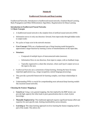
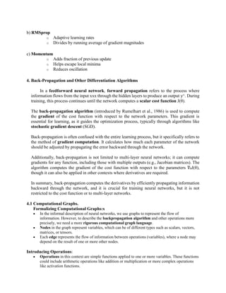
1.4 Activation Functions
1. Sigmoid (Logistic)
o Formula: σ(x) = 1/(1 + e^(-x))
o Range: [0,1]
o Used in binary classification
o Properties:
 Smooth gradient
 Clear prediction probability
 Suffers from vanishing gradient
2. Hyperbolic Tangent (tanh)
o Formula: tanh(x) = (e^x - e^(-x))/(e^x + e^(-x))
o Range: [-1,1]
o Often performs better than sigmoid
o Properties:
 Zero-centered
 Stronger gradients
 Still has vanishing gradient issue
3. ReLU (Rectified Linear Unit)
o Formula: f(x) = max(0,x)
o Most commonly used
o Helps solve vanishing gradient problem
o Properties:
 Computationally efficient
 No saturation in positive region
 Dying ReLU problem
4. Leaky ReLU
o Formula: f(x) = max(0.01x, x)
o Addresses dying ReLU problem
o Small negative slope
o Properties:
 Never completely dies
 Allows for negative values
 More robust than standard ReLU

4. 2 The XOR Problem
 Definition:
o XOR (exclusive OR) is a logical operation that outputs 1 (true) if and only if the
inputs differ.
o In other words:
 XOR(0, 0) = 0
 XOR(0, 1) = 1
 XOR(1, 0) = 1
 XOR(1, 1) = 0
 Challenge for Single-Layer Perceptrons:
o Single-layer perceptrons can only learn linearly separable functions.
o The XOR problem is not linearly separable.
o This means it's impossible to draw a single straight line to perfectly separate the
input points (0,0), (0,1), (1,0), (1,1) based on their XOR outputs.
The Power of Multi-Layer Perceptrons
 Non-linearity: Multi-layer perceptrons, with their hidden layers and non-linear activation
functions, can learn complex, non-linear decision boundaries.
 Solving XOR:
o A simple two-layer perceptron with a hidden layer can effectively solve the XOR
problem.
o The hidden layer learns to represent non-linear combinations of the inputs,
enabling the network to create a decision boundary that correctly classifies all
four input points.
Key Takeaways:
 The XOR problem demonstrates the limitations of single-layer perceptrons and highlights
the importance of non-linearity in neural networks.
 Multi-layer perceptrons with hidden layers can learn complex, non-linear functions,
making them powerful models for a wide range of tasks.
2. In essence: The XOR problem serves as a classic example to illustrate the need for hidden
layers and non-linear activation functions in neural networks to learn complex patterns and
solve non-linearly separable problems.
3. Gradient-Based Learning
 Gradient Descent: Neural networks are typically trained using gradient-based
optimization algorithms, similar to other machine learning models.
 Non-Convexity: The primary difference lies in the non-convexity of the loss function for
neural networks. This implies that gradient descent may find local minima rather than the
global minimum, making the training process more challenging.

5.  Parameter Initialization: Proper initialization of weights (small random values) is
crucial for successful training.
 Backpropagation: The core algorithm for efficiently computing gradients in neural
networks.
 Cost Function and Output Representation: Choosing an appropriate cost function and
output representation are critical design decisions in neural network training.
Comparison to Other Models:
 Linear Models: Trained using linear equation solvers or convex optimization algorithms
with strong convergence guarantees.
 Gradient Descent Applicability: Gradient descent can also be used to train linear
models, especially with large datasets.
In essence: While the underlying principle of gradient descent remains the same, training neural
networks presents unique challenges due to the non-convex nature of the optimization problem.
Understanding Gradients
1. Definition
o Gradient is a vector of partial derivatives
o Points in direction of steepest increase
o Used to minimize loss function
2. Properties
o Direction indicates fastest increase
o Magnitude indicates steepness
o Negative gradient used for minimization
3.2 Cost Functions
Definition of Cost Functions
 A cost function (also called a loss function in some contexts) measures how well or poorly a
model’s predictions align with the actual target values in the dataset. The goal of training a model
is to minimize this cost function, thereby improving the model’s accuracy on the task.
 In the context of neural networks, the cost function provides a quantitative measurement of the
error made by the network, and we use this to adjust the weights of the network during training.
Role of Cost Functions in Training
 The cost function drives the optimization process during training by providing a numerical value
that indicates how far the current predictions are from the target outputs.
 In gradient-based learning, gradient descent is used to minimize the cost function by adjusting
the network’s parameters (weights and biases) iteratively. The gradient of the cost function with
respect to the network’s parameters is computed and used to update the parameters in the
direction that reduces the cost.

6. Examples of Cost Functions
 Mean Squared Error (MSE)
o MSE is commonly used for regression problems. It calculates the average of the squares
of the differences between predicted and true values. The formula for MSE for a single
data point is:
where yi is the true value and y^i is the predicted value. The model tries to minimize the
MSE during training.
 Cross-Entropy Loss (Log Loss)
o For classification problems, especially binary and multi-class classification, cross-
entropy loss is often used. It measures the difference between the true probability
distribution (target labels) and the predicted probability distribution output by the
network (often from a softmax function in multi-class cases).
o Binary Cross-Entropy
where yi is the true label (0 or 1), and y^i is the predicted probability of class 1.
o Categorical Cross-Entropy is used for multi-class classification tasks and is a
generalization of binary cross-entropy.
Cost Function Behavior
 The behavior of the cost function influences how easily and effectively the model can be trained.
A well-chosen cost function ensures that the model can find good solutions and converge during
training.
 Convexity is a key consideration for cost functions. For a convex cost function, there is a single
global minimum, which guarantees that gradient descent will find this optimal solution regardless
of the starting point. However, non-convex cost functions (which are common in deep learning)
have multiple local minima or saddle points, and gradient descent can get stuck in suboptimal
solutions.
 Despite the lack of global convergence guarantees in non-convex optimization problems,
gradient-based methods still work well in practice due to the use of good initialization
techniques and stochastic gradient descent (SGD), which helps to escape poor local minima.
Choosing the Right Cost Function
 The choice of the cost function depends on the specific task the neural network is being trained
for:

7. o For regression tasks, MSE is commonly used.
o For binary classification, binary cross-entropy is used.
o For multi-class classification, categorical cross-entropy is used.
 In some cases, more complex or specialized cost functions may be used, such as those based on
focal loss or hinge loss (for support vector machines).
Regularization and Cost Functions
 Regularization is a technique used to prevent overfitting by adding a penalty term to the cost
function. Regularization terms are designed to discourage overly complex models by penalizing
large weights.
o L2 regularization (Ridge regression): Adds a penalty proportional to the sum of the
squared weights. The new cost function becomes:
where λ is a hyperparameter that controls the strength of the regularization.
o L1 regularization (Lasso regression): Adds a penalty proportional to the sum of the
absolute values of the weights. This often leads to sparse models with some weights
being exactly zero.
The Importance of Cost Functions in Optimization
 The cost function is central to the model's ability to generalize to new data. If the cost function is
well-designed and appropriate for the task, the model can learn effectively and perform well on
unseen data.
 The optimization algorithm, such as stochastic gradient descent (SGD), relies on the cost
function to determine how to update the parameters to reduce the error.
 Mini-batch gradient descent and variants (like Adam and RMSprop) are commonly used for
deep learning models because they help balance computational efficiency with effective
convergence during training.
Summary
 The cost function plays a critical role in training a neural network. It quantifies the error between
the predicted and actual values, guiding the optimization process to improve the model’s
performance.
 Different types of tasks (regression, binary classification, multi-class classification) require
different types of cost functions, such as MSE for regression or cross-entropy for classification.
 Regularization techniques, such as L1 and L2 regularization, are often added to the cost function
to prevent overfitting and ensure the model generalizes well to new data.
 The choice of cost function and the optimization algorithm used to minimize it are fundamental to
the success of training deep learning models.
This section outlines the importance of cost functions and their pivotal role in the learning
process of neural networks. By choosing an appropriate cost function and using optimization
techniques to minimize it, we can train models to solve a wide range of machine learning tasks.

8. 1. Mean Squared Error (MSE)
o Used for regression problems
o Formula: MSE = (1/n)Σ(y_true - y_pred)²
o Properties:
 Always positive
 Penalizes larger errors more
 Differentiable
2. Cross-Entropy Loss
o Used for classification problems
o Formula: -Σ(y_true * log(y_pred))
o Properties:
 Measures probability distribution difference
 Better for classification than MSE
 Provides stronger gradients
3. Huber Loss
o Combines MSE and MAE
o Less sensitive to outliers
o Formula:
 L = 0.5(y - f(x))² if |y - f(x)| ≤ δ
 L = δ|y - f(x)| - 0.5δ² otherwise
3.3 Gradient Descent Types
1. Batch Gradient Descent
o Uses entire dataset for each update
o More stable but slower
o Formula: θ = θ - α∇J(θ)
o Memory intensive for large datasets
2. Stochastic Gradient Descent (SGD)
o Updates parameters after each sample
o Faster but less stable
o Better for large datasets
o High variance in parameter updates
3. Mini-batch Gradient Descent
o Compromise between batch and SGD
o Updates parameters after small batches
o Most commonly used in practice
o Typical batch sizes: 32, 64, 128
4. Advanced Optimizers a) Adam (Adaptive Moment Estimation)
o Combines momentum and RMSprop
o Adaptive learning rates
o Formula includes first and second moments

9. b) RMSprop
o Adaptive learning rates
o Divides by running average of gradient magnitudes
c) Momentum
o Adds fraction of previous update
o Helps escape local minima
o Reduces oscillation
4. Back-Propagation and Other Differentiation Algorithms
In a feedforward neural network, forward propagation refers to the process where
information flows from the input xxx through the hidden layers to produce an output y^. During
training, this process continues until the network computes a scalar cost function J(θ).
The back-propagation algorithm (introduced by Rumelhart et al., 1986) is used to compute
the gradient of the cost function with respect to the network parameters. This gradient is
essential for learning, as it guides the optimization process, typically through algorithms like
stochastic gradient descent (SGD).
Back-propagation is often confused with the entire learning process, but it specifically refers to
the method of gradient computation. It calculates how much each parameter of the network
should be adjusted by propagating the error backward through the network.
Additionally, back-propagation is not limited to multi-layer neural networks; it can compute
gradients for any function, including those with multiple outputs (e.g., Jacobian matrices). The
algorithm computes the gradient of the cost function with respect to the parameters ∇θJ(θ),
though it can also be applied in other contexts where derivatives are required.
In summary, back-propagation computes the derivatives by efficiently propagating information
backward through the network, and it is crucial for training neural networks, but it is not
restricted to the cost function or to multi-layer networks.
4.1 Computational Graphs.
Formalizing Computational Graphs:s
 In the informal description of neural networks, we use graphs to represent the flow of
information. However, to describe the backpropagation algorithm and other operations more
precisely, we need a more rigorous computational graph language.
 Nodes in the graph represent variables, which can be of different types such as scalars, vectors,
matrices, or tensors.
 Each edge represents the flow of information between operations (variables), where a node may
depend on the result of one or more other nodes.
Introducing Operations:
 Operations in this context are simple functions applied to one or more variables. These functions
could include arithmetic operations like addition or multiplication or more complex operations
like activation functions.

10.  Operations are defined to produce single outputs. While in some cases operations might have
multiple outputs (such as vectors or matrices), this simplified model avoids such complexity for
clarity and conceptual understanding.
 Each operation will take variables as inputs and produce a result (output). For example, if a
variable yyy is computed by applying an operation to another variable xxx, the graph will have a
directed edge from xxx to yyy, indicating that yyy depends on xxx.
Graph Structure:
 The edges of the graph represent dependencies between variables. A directed edge from xxx to
yyy means that yyy is computed using xxx.
 Some computational graphs may annotate the output node with the name of the operation
applied (e.g., "addition," "multiplication"), but this is often omitted if the operation is clear from
context.
Simplification:
 To keep the explanation conceptual and straightforward, the authors focus on operations that
return a single output. Although many real-world implementations support operations with
multiple outputs, this detail is considered unnecessary for understanding the core idea of
computational graphs.
Examples of Computational Graphs:
 Refer to figure to show visual examples of how these graphs are structured, where nodes
represent variables and edges show the dependencies or flow of information. The figure likely
illustrates the flow of data through simple operations like multiplication, addition, and activation
functions.

11. 4.2 The Chain Rule in Calculus
 The chain rule is a basic concept in calculus that allows us to compute the derivative of a
composite function. If a function y is composed of several other functions, say y=f(g(x)), the
chain rule states that:
 In simpler terms, the chain rule says that the derivative of y with respect to x is the
product of the derivative of y with respect to g, and the derivative of g with respect to x.
 The chain rule can be extended to functions with multiple layers of composition, which is
exactly what we encounter in neural networks.
Application of the Chain Rule to Neural Networks
 In a neural network, each layer’s output depends on the inputs to the layer, and the output of each
layer is then passed to the next layer.
 Forward pass: In the forward pass of a neural network, the network computes the activations of
neurons layer by layer, moving forward through the network.
 Backward pass (Backpropagation): During backpropagation, we compute the gradients of the
loss with respect to the network's weights. Since the network's output depends on the weights and
activations of all preceding layers, we use the chain rule to compute these gradients efficiently.
Using the Chain Rule in Backpropagation
 To update the weights during training, we need the gradient of the cost function J with respect to
each weight w.
 Gradient computation involves applying the chain rule layer by layer, from the output of the
network back to the input.
o For instance, if the cost function J depends on the output y, and y is computed as a
function of z (the pre-activation in a layer), and z depends on the weights www, then:
 This chain of derivatives breaks down the gradient computation into smaller, manageable parts,
allowing the gradients to be computed efficiently.
Generalization of the Chain Rule
 The chain rule can be generalized to functions with multiple inputs and outputs. For example, if a
function has more than one input or output variable, the gradient must be computed for each of
these variables.
 In neural networks, this generalization is used to compute the gradient with respect to the weights
and biases of each layer, propagating the gradients backward through the network.

12. Gradient Flow
 The gradients computed using the chain rule indicate how the weights should be adjusted during
training. The gradients are propagated backward through the network, starting from the output
layer and moving toward the input layer.
 Each layer adjusts its weights based on how much they contributed to the error (calculated using
the gradient), ensuring that the network learns to minimize the cost function.
The chain rule of calculus is a key mathematical tool for computing the gradients used in
backpropagation. By applying the chain rule to the functions that define a neural network, we
can compute the gradient of the cost function with respect to each weight in the network. This
allows us to update the network's weights and minimize the cost function, which is the core of
the learning process in neural networks.
Recursively Applying the Chain Rule to Obtain Backprop
Key Concepts:
 Neural Networks as Function Composition: A neural network can be viewed as a
series of nested functions. Each layer performs a transformation on its input, and the
output of one layer serves as the input to the next.
 Chain Rule Application: The chain rule allows us to break down the complex gradient
calculation into a series of simpler steps.
o We calculate the local gradient at each node (operation) in the computational
graph.
o These local gradients are then combined recursively according to the chain rule to
obtain the gradient of the final output (cost function) with respect to any
parameter in the network.
Example:
Imagine a simple three-layer network:
1. Input Layer: Receives input 'x'.
2. Hidden Layer 1: Applies a linear transformation (Wx + b) followed by an activation
function (e.g., ReLU).
3. Hidden Layer 2: Applies another linear transformation and activation.
4. Output Layer: Produces the final output 'y'.
 To compute the gradient of the cost function with respect to the weights in the first layer:
o We first calculate the gradient of the cost with respect to the output of the last
layer.
o Then, we recursively apply the chain rule to calculate the gradient with respect to
the output of the previous layer, and so on, all the way back to the first layer.
 Backpropagation relies heavily on the recursive application of the chain rule.
 This recursive process allows for efficient computation of gradients across multiple
layers of a neural network. Understanding this recursive application of the chain rule is crucial
for grasping the core mechanics of backpropagation.

13. Key Steps:
1. Initialization:
o The algorithm starts with n_i input nodes, which are initialized with the input
vector x. These are the first n_i nodes in the graph.
2. Forward Computation:
o The algorithm iterates through the remaining nodes in the graph.
o For each node i:
 It identifies the set of parent nodes Pa(u(i)), which are the nodes that
provide input to node i.
 It collects the values of these parent nodes into a set A(i).
 It applies the operation f(i) to the set of arguments A(i) to compute the
value of node i.
3. Output:
o After processing all nodes, the algorithm returns the value of the output node
u(n).
In simpler terms:
Imagine the computational graph as a network of interconnected nodes. This algorithm starts at
the input nodes, calculates the values of each node based on the values of its parent nodes and
the associated operation, and finally reaches the output node, providing the final result of the
computation.
Example:
Consider a simple graph with three nodes:
 Node 1: Input node, initialized with value x.

14.  Node 2: Applies the operation f(2)(x) = x + 2 to the value of node 1.
 Node 3: Applies the operation f(3)(x) = 2 * x to the value of node 2.
In this case, the algorithm would:
1. Initialize node 1 with the input value x.
2. Calculate the value of node 2 as f(2)(x) = x + 2.
3. Calculate the value of node 3 as f(3)(x) = 2 * (x + 2).
The output of the graph would be the value of node 3, which is 2 * (x + 2).
Note: This algorithm forms the basis for performing forward passes in neural networks, where
the nodes represent operations like linear transformations, activation functions, and the flow of
data through the network.
Key Points:

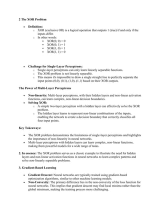
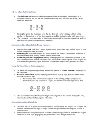
15.  Purpose: The algorithm aims to efficiently compute the gradient of the output node (u(n))
with respect to all other nodes (u(1), ..., u(n-1)) in the graph.
 Assumptions:
o All variables are scalars for simplicity.
o The computational cost of calculating the partial derivative associated with each
edge in the graph is assumed to be constant.
 Steps:
1. Forward Pass:
 The algorithm first performs a forward pass (using Algorithm 6.1) to
compute the activations of all nodes in the graph. This step is crucial as
the values of the nodes are required for the subsequent gradient
calculations.
2. Initialization:
 A data structure called grad_table is initialized.
 grad_table[u(n)] is set to 1, indicating that the gradient of the output node
with respect to itself is 1.
3. Backward Pass:
 The algorithm iterates backward through the nodes in the graph, starting
from the output node (n) and moving towards the input nodes.
 For each node j:
 The gradient of the output node (u(n)) with respect to node j
(du(n)/du(j)) is computed using the chain rule. This involves
summing the products of the gradients of the output node with
respect to its child nodes (u(i) where j is a parent of i) and the
partial derivatives of the child nodes with respect to node j.
 The calculated gradient is stored in grad_table[u(j)].
4. Output:
 The algorithm returns the grad_table, which contains the gradients of the
output node with respect to all other nodes in the graph.
In Essence:
Algorithm 6.2 demonstrates the core idea of backpropagation: recursively applying the chain rule
to efficiently compute gradients within a computational graph. By iterating backward through the
graph and utilizing the chain rule, the algorithm determines how changes in each node affect the
final output.
Note: This is a simplified version. The actual backpropagation algorithm in neural networks
would involve computing gradients with respect to the model's parameters (weights and biases),
which would require additional steps and considerations.
Back-Propagation Computation in Fully-Connected MLP
Key Concepts:
 Fully-Connected MLP: A neural network where each neuron in a layer is connected to
every neuron in the preceding layer.

16.  Backpropagation: The core algorithm for training neural networks. It efficiently
computes the gradient of the cost function with respect to the model's parameters
(weights and biases).
 Chain Rule: Backpropagation leverages the chain rule of calculus to recursively
compute the gradient for each layer, starting from the output layer and moving backward
through the network.
Process:
1. Forward Pass:
o The input data is fed forward through the network, layer by layer.
o At each layer, the weighted sum of the inputs is calculated, followed by the
application of an activation function (e.g., sigmoid, ReLU).
o The output of each layer is passed as input to the next layer.
2. Backward Pass:
o The error signal (difference between the network's output and the target output) is
calculated.
o The error signal is then propagated backward through the network.
o At each layer, the gradient of the error with respect to the weights and biases of
that layer is computed using the chain rule.
o These gradients are used to update the parameters of the network using an
optimization algorithm like gradient descent.
Example (Simplified):
Consider a simple two-layer MLP:
 Input Layer: Receives input vector x.
 Hidden Layer: Applies a linear transformation (Wx1 + b1) followed by an activation
function f1.
 Output Layer: Applies a linear transformation (Wx2 + b2) followed by an activation
function f2.
To compute the gradient of the cost function with respect to the weights and biases of the hidden
layer:
1. Calculate the gradient of the cost with respect to the output of the output layer.
2. Apply the chain rule to calculate the gradient with respect to the weights and biases of the
output layer.
3. Apply the chain rule again to calculate the gradient with respect to the output of the
hidden layer.
4. Finally, apply the chain rule to calculate the gradient with respect to the weights and
biases of the hidden layer.
In Essence:
Backpropagation in a fully-connected MLP involves recursively applying the chain rule to
efficiently compute the gradients of the cost function with respect to the parameters of each

17. layer. This allows the network to learn and adjust its parameters to minimize the error and
improve its performance.
Key Takeaways:
 Backpropagation is a fundamental algorithm for training neural networks.
 It enables efficient computation of gradients in multi-layer perceptrons.
 The chain rule plays a crucial role in the backpropagation process.
Note: This is a simplified explanation. The book provides a more detailed and mathematically
rigorous derivation of the backpropagation algorithm for fully-connected MLPs.
Purpose:
 To calculate the output of a deep neural network given an input.
 To compute the value of the cost function (loss) associated with the given input and
target output.
Inputs:
 l: Network depth (number of layers).
 W(i): Weight matrices for each layer i (from 1 to l).
 b(i): Bias vectors for each layer i (from 1 to l).

18.  x: The input to the network.
 y: The target output.
Steps:
1. Initialization:
o h(0) is set to the input x.
2. Forward Pass:
o The algorithm iterates through each layer k from 1 to l:
 a(k) is calculated as the weighted sum of the previous layer's output (h(k-1))
plus the bias vector (b(k)): a(k) = b(k) + W(k) * h(k-1).
 h(k) is calculated by applying the activation function f to a(k): h(k) = f(a(k)).
3. Output Calculation:
o The final output of the network is y^ = h(l).
4. Cost Function Calculation:
o The loss L(y^, y) is computed based on the difference between the predicted output
y^ and the target output y (examples of loss functions are given in section 6.2.1.1).
o The total cost J is calculated by adding the loss L(y^, y) to a regularization term
λΩ(θ), where λ is the regularization strength and Ω(θ) is the regularization function
(e.g., L2 regularization). θ represents all the model parameters (weights and
biases).
In Essence:
Algorithm 6.3 outlines the forward propagation process in a deep neural network. It shows how
the input is processed through each layer, with the output of one layer serving as the input to the
next. Finally, the algorithm calculates the cost associated with the network's output compared to
the target output.
Note: This algorithm provides a simplified view for a single input example. In practice, training
typically involves using minibatches of data for more efficient training.
Symbol-to-Symbol Derivatives
Key Concepts:
 Symbolic Differentiation: This section introduces the concept of symbolic
differentiation, which is a more general approach to computing derivatives compared to
the specific implementation of backpropagation for neural networks.
 Computational Graphs as a Foundation: Symbolic differentiation relies heavily on the
representation of computations using computational graphs.
 General Approach:
o Symbolic differentiation systems operate on the symbolic representation of the
function (defined by the computational graph).
o They apply the chain rule and other differentiation rules directly to the symbolic
expressions.
o This results in a symbolic expression for the gradient of the function.

19. o This symbolic expression can then be evaluated numerically for specific input
values.
Advantages of Symbolic Differentiation:
 Efficiency for Complex Functions: For complex functions with many repeated sub-
expressions, symbolic differentiation can be more efficient than numerical methods like
backpropagation. This is because common sub-expressions are only differentiated once
and then reused.
 Higher-Order Derivatives: Symbolic differentiation can easily compute higher-order
derivatives, which may be required for certain optimization algorithms or analysis
techniques.
Purpose:
 To compute the gradients of the cost function (loss) with respect to the model's
parameters (weights and biases) in a deep neural network.
 These gradients are then used to update the parameters using optimization algorithms like
stochastic gradient descent.

20. Inputs:
 The output of the forward pass (Algorithm 6.3), including the activations of each layer
(h(k)), the predicted output (y^), and the computed cost (J).
 The target output (y).
 Network depth (l), weights (W(k)), biases (b(k)), regularization strength (λ), and
regularization function (Ω(θ)).
Steps:
1. Initialize Gradient on Output Layer:
o The gradient of the cost function with respect to the output layer (g) is initialized
based on the derivative of the loss function (L(y, y^)).
2. Backward Pass:
o The algorithm iterates backward through the layers, starting from the output layer
(k = l) and going down to the first hidden layer (k = 1).
o For each layer k:
 Convert Gradient: The gradient on the layer's output is converted into a
gradient on the pre-nonlinearity activation (a(k)) using the derivative of the
activation function (f'(a(k))). This is typically done element-wise.
 Compute Gradients on Weights and Biases: The gradients of the cost
function with respect to the weights (W(k)) and biases (b(k)) of the current
layer are computed. This includes the contribution from the regularization
term.
 Propagate Gradients: The gradient is propagated to the activations of the
previous layer (h(k-1)).
3. Output:
o The algorithm returns the gradients of the cost function with respect to all weights
and biases in the network.
In Essence:
Algorithm 6.4 outlines the core backpropagation process. It shows how the error signal is
propagated backward through the network, allowing the model to learn and adjust its parameters
to minimize the cost function.
Key Takeaways:
 Backpropagation is a crucial algorithm for training deep neural networks.
 It efficiently computes the gradients of the cost function with respect to the model's
parameters.
 The algorithm leverages the chain rule to propagate the error signal backward through the
network.
Note: This algorithm provides a simplified view. In practice, there are various optimization
techniques and regularization methods that can be integrated into the backpropagation process to
improve training efficiency and generalization.

21. Key Points:
 Symbolic vs. Numerical Differentiation:
o Numerical Differentiation: Traditionally, gradients are computed numerically
using finite differences (e.g., approximating the derivative by a small change in
the input).
o Symbolic Differentiation: This approach operates directly on the symbolic
representation of the function (defined by the computational graph). It applies
differentiation rules (like the chain rule) to derive a symbolic expression for the
gradient.
 Figure :
o Left: Shows a simple computational graph representing a function z = f(f(f(w))).
o Right: Shows the result of applying symbolic differentiation.
 The graph is augmented with nodes representing the derivatives.
 The arrows now indicate how these derivatives are computed and
combined using the chain rule.
 Benefits of Symbolic Differentiation:
o Efficiency: If the same function is evaluated and differentiated multiple times,
symbolic differentiation can be more efficient. This is because the symbolic
expression for the gradient is computed only once and then reused for different
input values.
o Higher-Order Derivatives: Symbolic differentiation can easily compute higher-
order derivatives (e.g., second derivatives), which are required for certain
optimization algorithms and analysis techniques.
In Essence:
Figure illustrates the core principle of symbolic differentiation: transforming a computational
graph representing a function into a new graph that represents the derivative of that function.
This approach provides a powerful and general way to compute gradients and enables more
efficient and flexible gradient-based optimization.

22. Note: Although Figure is not directly visible, the description provides a clear understanding of
its purpose and the key concepts of symbolic differentiation.
General Back-Propagation
Key Concepts:
 Extending Backpropagation: This section moves beyond the specific case of fully-
connected feedforward networks and discusses how backpropagation can be applied to
more general computational graphs.
 Computational Graphs as the Foundation: The concept of computational graphs is
central. Any differentiable computation, regardless of its specific form, can be
represented as a computational graph.
 Generic Backpropagation Algorithm: The core idea is to derive a general
backpropagation algorithm that can operate on any arbitrary computational graph.
o This algorithm would traverse the graph, applying the chain rule at each node to
compute the gradients of the output with respect to the input variables.
Key Takeaways:
 Backpropagation is not limited to specific neural network architectures.
 It can be applied to any differentiable computation that can be represented as a
computational graph.
 This generality makes backpropagation a powerful tool for a wide range of machine
learning and other applications.
Example:
 While the initial examples focus on feedforward neural networks, the principles of
backpropagation can be extended to:
o Recurrent Neural Networks (RNNs)
o Convolutional Neural Networks (CNNs)
o More complex architectures involving recurrent connections, memory units, and
other sophisticated components.
Computing Gradients:
 The process starts by recognizing that the gradient of a variable z with respect to itself
(dz/dz) is 1.
 To compute the gradient of z with respect to its parent node y:
o Calculate the Jacobian of the operation that produced z (i.e., how a small change
in y affects z).
o Multiply the current gradient (dz/dz) by this Jacobian.
 This process continues recursively, moving backward through the graph.
 If a node has multiple parents, the gradients from all paths are summed to obtain the total
gradient for that node.

23. Purpose:
 This algorithm provides the overall framework for computing gradients of a target set of
variables (T) with respect to other variables in a computational graph.
Inputs:
 T: The set of target variables for which we want to compute the gradients.
 G: The computational graph representing the relationships between variables.
 z: The variable to be differentiated (usually the output of the graph or the cost function).
Steps:

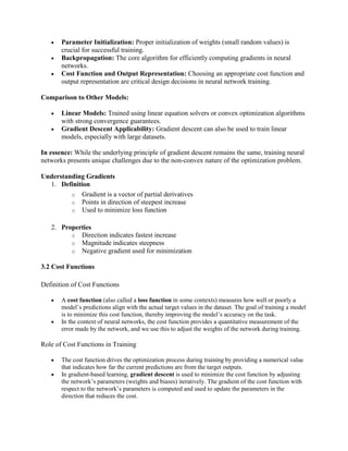
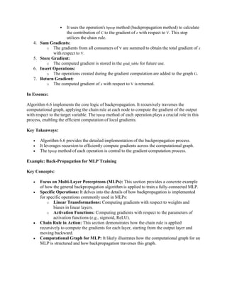
24. 1. Graph Pruning:
o The algorithm creates a pruned subgraph G' from the original graph G.
o G' only includes nodes that are:
 Ancestors of z (nodes that contribute to the calculation of z).
 Descendants of nodes in T (nodes that are affected by the target variables).
o This pruning step reduces the computational complexity by focusing only on the
relevant parts of the graph.
2. Initialization:
o A data structure grad_table is initialized. This table will store the computed
gradients for each variable.
o grad_table[z] is set to 1, as the gradient of z with respect to itself is 1.
3. Gradient Computation:
o The algorithm iterates over each target variable V in the set T.
o For each target variable V, it calls the build_grad subroutine (Algorithm 6.6, not
shown here). This subroutine performs the core backpropagation calculations to
compute the gradient of z with respect to V.
4. Output:
o The algorithm returns the grad_table, which now contains the computed gradients
of z with respect to the target variables in T.
Key Takeaways:
 Algorithm 6.5 provides the overall structure and workflow of the backpropagation
process.
 It highlights the importance of graph pruning to improve efficiency.
 It delegates the core gradient computation to the build_grad subroutine (Algorithm 6.6),
which likely implements the recursive application of the chain rule.
In Essence:
Algorithm 6.5 serves as the high-level framework for backpropagation. It establishes the context,
initializes the necessary data structures, and orchestrates the gradient computation for the target
variables. The actual computation of gradients is delegated to the build_grad subroutine, which
will be discussed in detail in Algorithm 6.6.
Algorithm 6.6: Backpropagation - build_grad Subroutine
Purpose:
 This subroutine is responsible for computing the gradient of the output variable (z) with
respect to a specific target variable (V) within the computational graph.
 It is called by the outer backpropagation algorithm (Algorithm 6.5) for each target
variable.

25. Inputs:
 V: The target variable whose gradient needs to be computed.
 G: The full computational graph.
 G': The pruned subgraph containing only nodes relevant to the computation of the
gradient of z with respect to V.
 grad_table: A data structure to store computed gradients.
Steps:
1. Check if Gradient is Already Computed:
o If the gradient of z with respect to V is already stored in the grad_table, the
algorithm simply returns the stored value.
2. Iterate over Consumers:
o The algorithm iterates through all the "consumers" of V. Consumers are nodes in
the graph that take V as an input.
3. Compute Child Gradients:
o For each consumer C:
 It retrieves the operation associated with node C.
 It recursively calls build_grad to compute the gradient of z with respect to C.

26.  It uses the operation's bprop method (backpropagation method) to calculate
the contribution of C to the gradient of z with respect to V. This step
utilizes the chain rule.
4. Sum Gradients:
o The gradients from all consumers of V are summed to obtain the total gradient of z
with respect to V.
5. Store Gradient:
o The computed gradient is stored in the grad_table for future use.
6. Insert Operations:
o The operations created during the gradient computation are added to the graph G.
7. Return Gradient:
o The computed gradient of z with respect to V is returned.
In Essence:
Algorithm 6.6 implements the core logic of backpropagation. It recursively traverses the
computational graph, applying the chain rule at each node to compute the gradient of the output
with respect to the target variable. The bprop method of each operation plays a crucial role in this
process, enabling the efficient computation of local gradients.
Key Takeaways:
 Algorithm 6.6 provides the detailed implementation of the backpropagation process.
 It leverages recursion to efficiently compute gradients across the computational graph.
 The bprop method of each operation is central to the gradient computation process.
Example: Back-Propagation for MLP Training
Key Concepts:
 Focus on Multi-Layer Perceptrons (MLPs): This section provides a concrete example
of how the general backpropagation algorithm is applied to train a fully-connected MLP.
 Specific Operations: It delves into the details of how backpropagation is implemented
for specific operations commonly used in MLPs:
o Linear Transformations: Computing gradients with respect to weights and
biases in linear layers.
o Activation Functions: Computing gradients with respect to the parameters of
activation functions (e.g., sigmoid, ReLU).
 Chain Rule in Action: This section demonstrates how the chain rule is applied
recursively to compute the gradients for each layer, starting from the output layer and
moving backward.
 Computational Graph for MLP: It likely illustrates how the computational graph for an
MLP is structured and how backpropagation traverses this graph.

27. Complications
Numerical Instability:
 Vanishing/Exploding Gradients: In deep networks, gradients can become extremely
small (vanishing) or extremely large (exploding) during backpropagation. This can hinder
the training process and make it difficult to learn.
 Techniques to address these issues, such as gradient clipping and careful initialization
strategies, are likely discussed.
Computational Efficiency:
 Implementing backpropagation efficiently is crucial for training large and complex neural
networks.
 The book might discuss optimization techniques for the backpropagation algorithm, such
as efficient memory management and parallel/distributed computation.
Higher-Order Derivatives:
 While backpropagation primarily focuses on first-order derivatives, some advanced
optimization algorithms or analysis techniques might require higher-order derivatives
(e.g., second-order derivatives for Newton's method).
 The section might discuss the challenges of computing higher-order derivatives using
backpropagation and alternative approaches.
Software Implementations:
 Practical considerations related to implementing backpropagation in software, such as
numerical stability issues, efficient memory management, and debugging techniques,
might be discussed.
Differentiation outside the Deep Learning Community
Key Concepts:
 Broader Applications of Differentiation: This section likely explores the broader
applications of differentiation techniques beyond the context of training neural networks.
 Scientific Computing: Differentiation plays a crucial role in various scientific
computing fields, such as:
o Physics and Engineering: Solving differential equations, numerical simulations,
and optimization problems in fields like fluid dynamics, structural mechanics, and
control systems.
o Computational Chemistry and Biology: Modeling and simulating molecular
dynamics, protein folding, and other complex biological processes.
o Finance: Risk management, option pricing, and portfolio optimization.
 Optimization: Differentiation is fundamental to many optimization algorithms, such as:
o Newton's Method: Uses second-order derivatives (Hessian matrix) for efficient
optimization.
o Constrained Optimization: Techniques like Lagrange multipliers and Karush-
Kuhn-Tucker (KKT) conditions rely on gradients and derivatives for finding
optimal solutions.
 Automatic Differentiation (AD): The principles of automatic differentiation, similar to
those used in backpropagation, have broader applications beyond deep learning.

28. AD tools can be used to efficiently compute derivatives for a wide range of functions and
models in various scientific and engineering domains.
Higher-Order Derivatives
Key Concepts:
 Beyond First-Order Derivatives: While most neural network training relies on first-
order derivatives (gradients) for optimization (e.g., gradient descent), some advanced
techniques utilize higher-order derivatives.
 Second-Order Derivatives (Hessian Matrix): The Hessian matrix is a matrix of second-
order partial derivatives. It provides information about the curvature of the cost
function.
 Newton's Method: This optimization algorithm uses the Hessian matrix (second-order
derivatives) to find the minimum of a function. It often converges faster than gradient
descent, especially near the minimum.
 Challenges with Higher-Order Derivatives:
o Computational Cost: Computing and storing the Hessian matrix can be
computationally expensive, especially for large neural networks.
o Numerical Instability: Computing and inverting the Hessian matrix can be
numerically unstable.
 Approximations:
o Due to the computational challenges, approximations to the Hessian matrix are
often used:
 Diagonal Approximation: Only the diagonal elements of the Hessian are
computed, which significantly reduces computational cost.
 Limited-Memory Quasi-Newton Methods: These methods approximate
the Hessian using information from previous gradient updates.
Historical Notes
1. Early History of Neural Networks:
 Perceptron: The early work on single-layer perceptrons and their limitations.
 Multi-Layer Perceptrons: The development of multi-layer perceptrons and the initial
challenges in training them.
2. The Backpropagation Revolution:
 The 1986 paper: The seminal paper by Rumelhart, Hinton, and Williams in 1986 that
introduced the backpropagation algorithm as we know it today.
 Impact of the 1986 paper: How this paper revitalized research in neural networks and
led to significant advancements in the field.
3. Early Challenges and Limitations:

29.  Vanishing/Exploding Gradients: The challenges associated with training deep
networks, such as vanishing and exploding gradients, and early attempts to address these
issues.
 Computational Limitations: The computational constraints of the time and how they
limited the progress of deep learning research.
4. Key Milestones:
 The rise of deep learning: The key breakthroughs and developments in the 2000s and
2010s that led to the resurgence of deep learning, including advancements in hardware,
algorithms, and datasets.
 Notable contributions: The contributions of key researchers and their influential work in
the field of deep learning.
Regularization for Deep Learning
Key Points:
 Overfitting: A common challenge in machine learning where a model performs well on
the training data but poorly on unseen data.
 Regularization: Techniques to improve generalization by reducing overfitting.
 Trade-off Between Bias and Variance: Regularization aims to find a balance between
bias (underfitting) and variance (overfitting).
 Regularization Strategies:
o Constraint on Model Complexity:
 Limiting the number of parameters (model size).
 Adding constraints or penalties to the model's parameters (e.g., weight
decay).
o Ensembling: Combining multiple models to improve generalization.
 Deep Learning and Model Complexity:
o Deep learning often involves complex models with a large number of parameters.
o Effective regularization is crucial to prevent overfitting in such models.
o The goal is to find the right balance of complexity and regularization to achieve
optimal generalization.
 Regularization is crucial for training effective deep learning models.
 It aims to find a balance between bias and variance.
 Deep learning often involves finding the right balance of model complexity and
regularization.
In essence:
This introductory section highlights the importance of regularization in deep learning. It explains
that while complex models are powerful, they are prone to overfitting. Regularization techniques
are essential to control model complexity, prevent overfitting, and improve generalization
performance on unseen data.

30. Parameter Norm Penalties
 Objective Function: Regularization is often achieved by adding a penalty term (Ω(θ)) to
the original cost function (J(θ)).
 Regularization Strength: The hyperparameter α controls the strength of the
regularization. A higher α value indicates stronger regularization.
 Focus on Weights: Typically, only the weights of the affine transformations in each
layer are penalized, while biases are left unregularized. This is because biases generally
require less data to fit accurately compared to weights.
Different Norms:
 The choice of the norm function (Ω(θ)) influences the behaviour of the regularization.
 The passage mentions that different norms will result in different solutions and
regularization effects.
 Regularization is crucial for improving the generalization ability of deep learning models.
 Parameter norm penalties, such as L2 regularization, are effective techniques for
controlling model complexity.
 The choice of the norm function and the regularization strength are important
hyperparameters that influence the model's performance.
L2 Parameter Regularization
Key Concepts:
 L2 Regularization (Weight Decay):
o Adds a penalty term to the cost function that is proportional to the sum of the
squares of the weights.
o Mathematically: J(θ) = L(θ) + λ ||θ||₂² where L(θ) is the original loss, λ is
the regularization strength, and ||θ||₂² is the squared L2 norm of the weights.
 Effect on Weights:
o Encourages the model to learn smaller weights.
o Reduces the model's sensitivity to small fluctuations in the input data.
 Gradient Update:
o Modifies the gradient update rule to include a weight decay term: w ← w - α *
(∇L(θ) + 2λw).
 Analysis with Quadratic Approximation:
o Approximates the cost function around the minimum of the unregularized cost
function with a quadratic function.
o Analyzes how L2 regularization affects the optimal solution in this simplified
scenario.
 Connection to Linear Regression:
o Demonstrates how L2 regularization affects the solution of linear regression.
o Shows that L2 regularization effectively increases the perceived variance of the
input features, leading to smaller weights for features with low covariance with
the output.
Key Equations:

31.  Regularized Objective Function: J˜(θ; X, y) = L(θ; X, y) + λ ||θ||₂²
 Gradient Update with L2 Regularization: w ← w - α * (∇L(θ) + 2λw)
 Normal Equations for Linear Regression with L2 Regularization:
αI)⁻
 L2 regularization is a fundamental technique for controlling model complexity and
preventing overfitting in deep learning.
 It encourages the learning of smaller weights, leading to improved generalization and
robustness.
 The mathematical analysis provides a deeper understanding of how L2 regularization
affects the learning process.
L1 Regularization (Lasso):
 Core Concept: L1 regularization, also known as Lasso, adds a penalty term to the cost
function that is proportional to the sum of the absolute values of the weights.
 Mathematical Formulation:
The cost function with L1 regularization takes the following form:
J(θ) = L(θ) + λ ||θ||₁
where:
o L(θ) is the original loss function (e.g., cross-entropy, mean squared error).
o λ is the regularization strength (a hyperparameter that controls the impact of the
penalty).
o ||θ||₁ is the L1 norm of the weights (sum of the absolute values of all weights).
 Effect on Weights:
o The L1 penalty encourages sparsity in the model, meaning many of the weights
will become exactly zero.
o This can be beneficial for feature selection, as it effectively removes irrelevant
features from the model.
 Gradient Update:
o The gradient of the L1 penalty term is non-differentiable at zero.
o In practice, approximations or techniques like subgradient descent are used to
handle this non-differentiability.
Key Takeaways:
 L1 regularization promotes sparsity in the model, leading to improved interpretability and
potential feature selection.
 It can be useful when the underlying data is believed to have a sparse representation.
 L1 regularization can be computationally more expensive than L2 regularization due to
the non-differentiability of the L1 norm at zero.
Norm Penalties as Constrained Optimization
 Equivalence of Penalties and Constraints:

32.  The authors likely demonstrate that adding a penalty term to the cost function (like in L1
or L2 regularization) is mathematically equivalent to imposing a constraint on the
model's parameters.
 For example, L2 regularization can be seen as imposing a constraint on the Euclidean
norm of the weight vector.
 Lagrangian Formulation:
 This section might introduce the Lagrangian formulation, a mathematical technique used
to solve constrained optimization problems.
 The Lagrangian combines the original objective function with a constraint function using
a Lagrange multiplier.
 Geometric Interpretation:
 The authors might provide a geometric interpretation of the effect of these constraints on
the optimization process.
 For example, L2 regularization can be visualized as projecting the solution onto a sphere
(or a hypersphere in higher dimensions) defined by the constraint on the norm of the
weights.
 Connection to Bias-Variance Trade-off:
 The section might discuss how these constraints affect the bias-variance trade-off.
 For example, constraints can limit the model's complexity, reducing variance but
potentially increasing bias.
 J(θ; X, y): This represents the original cost function or the loss function. It measures
the discrepancy between the model's predictions and the actual ground truth.
o θ: Represents the model's parameters (weights and biases).
o X: Represents the input data.
o y: Represents the corresponding target values or labels.

33.  Ω(θ): This term represents the regularization term. It penalizes large values of the
model's parameters. Common examples include:
o L1 regularization: Ω(θ) = ||θ||₁ (sum of the absolute values of the weights)
o L2 regularization: Ω(θ) = ||θ||₂² (sum of the squares of the weights)
 α: This is the regularization strength or the hyperparameter that controls the influence
of the regularization term. A higher value of α indicates stronger regularization.
 J˜(θ; X, y): This represents the regularized cost function. It combines the original loss
function with the regularization term.
Regularization and Under-Constrained Problems
X+ = lim_α→0 (X^TX + αI)^-1X^T
 X: The original matrix.
 X^T: The transpose of matrix X.
 I: The identity matrix.
 α: A small scalar value.
 lim_α→0: The limit as α approaches zero.
Interpretation:
1. X^TX + αI: This term is crucial. Adding αI to X^TX ensures
that the resulting matrix is invertible, even if X^TX itself is singular (i.e.,
does not have an inverse). This addition is essentially a form of regularization.
2. (X^TX + αI)^-1: The inverse of the regularized matrix
(X^TX + αI).
3. (X^TX + αI)^-1X^T: This part calculates the
pseudoinverse for a given value of α.
4. lim_α→0: As α approaches zero, the regularization effect diminishes. The
pseudoinverse X+ is the limit of this expression as α becomes infinitesimally small.
Significance:
 Handling Singular Matrices: The pseudoinverse allows us to work with matrices that don't have
a traditional inverse. This is particularly useful in situations where the number of rows is less than
the number of columns, or when the matrix is rank-deficient.
 Linear Regression: The pseudoinverse has a direct connection to linear regression. In linear
regression, we aim to find the best-fit line (or hyperplane) that minimizes the difference between
the predicted values and the actual values. 1
The pseudoinverse provides a way to compute the
optimal weights for the linear regression model, even when the data matrix (X) is not invertible.
 Regularization: The equation shows the connection between the pseudoinverse and
regularization. The addition of αI to X^TX can be seen as a form of regularization,
similar to L2 regularization, which helps to stabilize the solution and improve its robustness.

34. Dataset Augmentation
Key Concepts:
 Overfitting and Data Scarcity: Deep learning models, especially those with a large
number of parameters, are prone to overfitting, especially when the training dataset is
limited. Overfitting occurs when the model learns to perform well on the training data but
fails to generalize to unseen data.
 Data Augmentation as a Solution: Dataset augmentation addresses this issue by
creating modified versions of existing training data. This increases the size and diversity
of the training set without collecting new data.
 Techniques for Image Data: Common data augmentation techniques for image data
include:
o Geometric transformations: Rotating, flipping, scaling, cropping, shearing,
translating images.
o Color space manipulations: Adjusting brightness, contrast, saturation, and hue.
o Noise injection: Adding Gaussian noise, salt-and-pepper noise, or other types of
noise to the images.
 Techniques for Other Data Types:
o Text data: Word shuffling, synonym replacement, back-translation.
o Audio data: Adding noise, changing pitch, time-stretching.
o Time series data: Adding noise, time shifting, scaling.
 Benefits of Data Augmentation:
o Improved generalization: By exposing the model to a wider variety of data, data
augmentation helps the model learn more robust and generalizable features.
o Reduced overfitting: By increasing the effective size of the training set, data
augmentation helps to prevent the model from memorizing the training data.
o Reduced need for large datasets: Data augmentation can be used to effectively
train models on smaller datasets.
Noise Robustness
 Noise as Regularization:
 Adding noise to the input of a model can act as a form of regularization.
 In some cases, injecting infinitesimal noise at the input is mathematically equivalent to
applying an L2 weight decay penalty.
 Noise Injection at Hidden Units: Dropout
 Adding noise to the activations of hidden units during training is a powerful
regularization technique.
 Dropout, which randomly drops out neurons during training, can be viewed as a form of
noise injection at the hidden layer activations.
 Noise Injection to Weights:
 Adding noise to the model's weights during training can also improve generalization.

35.  This technique can be interpreted as a stochastic approximation to Bayesian inference,
where the weights are treated as uncertain variables.
 Weight noise can encourage the model to learn more stable and robust functions.
 Noise Injection and Stability:
 Adding noise to the weights can encourage the model to learn functions that are less
sensitive to small perturbations in the weights.
 This can be particularly beneficial in recurrent neural networks.
 Connection to Bayesian Inference:
 Adding noise to the weights reflects the uncertainty associated with the model parameters
in a Bayesian framework.
 Example: Regression with Weight Noise:
 The text sets the stage for further discussion by considering a regression setting where
noise is added to the weights.
 This example will likely demonstrate how weight noise can influence the learning
process and improve generalization in a specific context.
The equation you provided represents the expected value of the squared error or the mean
squared error (MSE), a common loss function used in regression tasks. Let's break it down:
 J: This symbol typically represents the cost function or loss function. It quantifies the
error between the model's predictions and the actual ground truth.
 E_p(x,y): This denotes the expectation operator. It means we are taking the
average of the following expression over all possible input-output pairs (x, y) drawn from
the data distribution p(x, y).
 ŷ(x): This represents the model's prediction for the input x. It's the output of the model
when input x is fed into it.
 y: This represents the actual ground truth or the target value corresponding to the input
x.
 (ŷ(x) - y)²: This is the squared error between the model's prediction and the actual
value. It measures the magnitude of the difference between the prediction and the true
value.

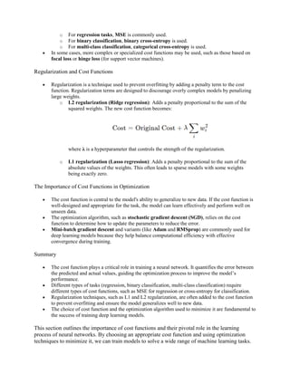
36. In summary:
The equation J = E_p(x,y)[(ŷ(x) - y)²] represents the mean squared error (MSE) loss
function. It calculates the average squared difference between the model's predictions and the
true values for all possible input-output pairs in the dataset. The goal during training is to
minimize this MSE loss function by adjusting the model's parameters.
Injecting Noise at the Output Targets
Key Points:
 Problem with Noisy Labels:
o Real-world datasets often contain errors or inaccuracies in the labels.
o Training a model directly on such noisy labels can lead to suboptimal
performance and overfitting.
 Label Smoothing:
o This technique addresses noisy labels by introducing "soft" targets instead of
hard, one-hot encoded labels.
o For a k-class classification problem, instead of using a one-hot vector (e.g., [0, 1,
0] for the second class), label smoothing replaces the 1 with (1 - ϵ) and distributes
the remaining probability mass (ϵ) equally among the other classes (e.g., [ϵ/k, 1 -
ϵ, ϵ/k]).
o Here, ϵ is a small constant.
 Benefits of Label Smoothing:
o Prevents Overfitting: By introducing uncertainty in the labels, label smoothing
prevents the model from becoming overly confident in its predictions and
encourages it to learn more robust representations.
o Improved Generalization: Label smoothing can lead to better generalization
performance on unseen data.
o Addresses the Issue of Hard Predictions: Softmax activations can never output
probabilities of exactly 0 or 1. Label smoothing helps to avoid this issue by
providing more realistic target distributions.
 Historical Context:
o Label smoothing has been used in machine learning for many years, dating back
to the 1980s.
o It continues to be a valuable technique in modern deep learning models, as
demonstrated by its use in architectures like Inception (Szegedy et al., 2015).
Semi-Supervised Learning
Key Concepts:
 Leveraging Unlabeled Data: Semi-supervised learning aims to improve the
performance of machine learning models by utilizing both labeled and unlabeled data.
 Representation Learning: A common approach in semi-supervised learning is to learn a
good representation (feature extraction) of the data. The goal is to learn a representation
where data points from the same class are mapped to similar representations in the feature
space.

37.  Unsupervised Learning as a Guide: Unsupervised learning techniques, such as
clustering or dimensionality reduction (e.g., PCA), can provide valuable information
about the underlying data structure and guide the learning process.
 Generative Models: Combining generative models (which model the data distribution
P(x)) with discriminative models (which model the conditional distribution P(y|x)) can be
effective. Shared parameters between these models can capture the relationship between
the data distribution and the classification task.
 Kernel Methods: Semi-supervised learning can also be applied to kernel methods, where
unlabeled data can be used to improve the kernel function and enhance the performance
of the classifier.
Multi-Task Learning
 Sharing Parameters: Multi-task learning leverages the idea of sharing parameters across
multiple tasks. This shared component of the model acts as a common ground, enforcing a
degree of similarity in the learned representations.
 Soft Constraints: The shared parameters can be seen as "soft constraints" on the model. They
encourage the model to learn features that are relevant to multiple tasks, leading to a more
generalizable and robust representation.
 Improved Generalization: By sharing information across tasks, multi-task learning can
improve the generalization performance of each individual task. This is because the shared
parameters are regularized by the constraints imposed by the other tasks.
 Data Efficiency: When data for individual tasks is limited, multi-task learning can be highly
beneficial. By learning from multiple tasks simultaneously, the model can effectively leverage
the information from all tasks, leading to improved performance even with limited data for each
individual task.

38.  Shared Representation: The central node labeled "h(shared)" represents a shared
representation layer. This layer extracts features from the input "x" that are relevant to
multiple tasks.
 Task-Specific Layers: The nodes labeled "h(1)", "h(2)", and "h(3)" represent task-
specific layers. These layers build upon the shared representation to perform the specific
tasks.
 Outputs: The nodes labeled "y(1)" and "y(2)" represent the outputs of the individual
tasks.
How it Works:
1. Input: The input "x" is fed into the network.
2. Shared Representation: The input is processed by the shared layer "h(shared)", which
extracts common features relevant to all tasks.
3. Task-Specific Processing: The shared representation is then passed to the task-specific
layers "h(1)", "h(2)", and "h(3)". Each of these layers further processes the features to
perform its respective task.
4. Output: Finally, each task-specific layer generates its own output, "y(1)" and "y(2)".
Benefits of this Architecture:
 Improved Generalization: By sharing the initial layers, the model learns features that
are relevant to multiple tasks, leading to better generalization for each individual task.
 Data Efficiency: The shared representation allows the model to learn from the data
associated with all tasks, even if the data for each individual task is limited.
 Regularization: The shared representation acts as a form of regularization, preventing
overfitting to any single task.
This is a simplified illustration, and real-world multi-task learning architectures can be more
complex, involving multiple shared layers, different levels of parameter sharing, and more
intricate connections between tasks.

39.  Training Loss: The training loss consistently decreases over time as the model learns to
fit the training data better. This is expected behavior during training.
 Validation Loss:
o Initially, the validation loss also decreases, indicating that the model is learning
generalizable features.
o However, after a certain point, the validation loss starts to increase again even
though the training loss continues to decrease.
Interpretation:
 Overfitting: This "U-shaped" curve is a classic sign of overfitting. The model has started
to memorize the training data too well, capturing noise and irrelevant details. As a result,
it performs poorly on unseen data (the validation set).
 Maxout Network: The fact that this is observed in a maxout network is not surprising.
Maxout networks, while powerful, can have a high capacity, making them more prone to
overfitting if not properly regularized.
Key Takeaways:
 Importance of Monitoring Validation Loss: The validation loss curve is crucial for
identifying overfitting and determining the optimal stopping point for training.
 Regularization Techniques: To prevent overfitting, regularization techniques like
dropout, weight decay, early stopping, and data augmentation are essential.
Early Stopping
 Concept: Early stopping is a simple yet effective regularization technique that monitors
the model's performance on a separate validation set during training.
 Procedure:
1. Divide the available data into training, validation, and (optionally) test sets.
2. Train the model on the training set.
3. After each training epoch (or at regular intervals), evaluate the model's
performance on the validation set.
4. Stop the training process when the validation performance starts to degrade, even
though the training loss may still be decreasing.
 Rationale:
o Overfitting occurs when the model starts to memorize the training data too well,
leading to poor generalization on unseen data.
o Early stopping detects this overfitting behavior by monitoring the performance on
the validation set.
o By stopping training before the model starts to overfit, early stopping helps to
maintain good generalization performance.
 Advantages:
o Simple to implement and computationally inexpensive.
o Does not require any modifications to the model architecture or the loss function.
o Can be effective in preventing overfitting in many deep learning models.
In Essence:

40. Early stopping is a practical and effective regularization technique that leverages the validation
set to identify and prevent overfitting. By monitoring the model's performance on unseen data
during training, early stopping helps to find the optimal balance between training error and
generalization performance.
Key Takeaways:
 Early stopping is a simple yet effective regularization technique.
 It monitors the model's performance on a validation set1
to detect overfitting.
 By stopping training early, it helps to prevent overfitting and improve generalization.
Purpose:
 This algorithm implements the early stopping technique to determine the optimal number
of training steps for a given model.
 It aims to prevent overfitting by stopping the training process before the model's
performance on unseen data (validation set) starts to degrade.
Inputs:
 n: The number of training steps between evaluations of the validation set error.

41.  p: The "patience" parameter, which determines how many consecutive times the
validation error can worsen before training is stopped.
Initialization:
 θ₀: The initial model parameters.
 i: The current training step (initialized to 0).
 j: A counter for the number of consecutive times the validation error has worsened.
 v: The current best validation error (initialized to infinity).
 θ*: The best model parameters found so far (initialized to θ₀).
 i*: The number of training steps at which the best validation error was achieved.
Training Loop:
1. Training: Update the model parameters (θ) by running the training algorithm for n steps.
2. Validation: Evaluate the model's performance on the validation set and calculate the
current validation error (v').
3. Check for Improvement:
o If the current validation error (v') is better than the previous best validation error
(v):
 Reset the counter j to 0.
 Update the best parameters (θ*) and the corresponding number of training
steps (i*) with the current values.
 Update the best validation error (v) with the current validation error (v').
o If the current validation error is worse than the previous best validation error:
 Increment the counter j by 1.
4. Stopping Condition: If the counter j exceeds the patience level p, stop training. The best
parameters (θ*) and the corresponding number of training steps (i*) represent the
optimal stopping point.
Output:
 θ*: The best model parameters found during training.
 i*: The optimal number of training steps before stopping.
Purpose:
 This algorithm aims to refine the early stopping strategy by using a two-step process.
 It first determines the optimal number of training steps using early stopping on a smaller
subset of the training data.

42.  Then, it retrains the model on the full training set for the determined number of steps.
Steps:
1. Data Splitting:
o Divide the original training set (X(train), y(train)) into two subsets:
 Training Subset: (X(subtrain), y(subtrain)) used for training and
monitoring performance during the initial early stopping phase.
 Validation Subset: (X(valid), y(valid)) used for validation during the
initial early stopping phase.
2. Initial Early Stopping:
o Run Algorithm 7.1 (the early stopping algorithm) using the training subset
(X(subtrain), y(subtrain)) for training and the validation subset (X(valid),
y(valid)) for validation.
o This step determines the optimal number of training steps (i*) before overfitting
starts to occur on the validation subset.
3. Retraining on Full Dataset:
o Reinitialize the model parameters to random values.
o Train the model on the entire training set (X(train), y(train)) for exactly i* steps,
the optimal number of steps determined in the previous step.
Key Advantages:
 Improved Generalization: By determining the optimal training duration on a smaller
subset and then retraining the model on the full dataset for that duration, this approach
can lead to improved generalization performance.
 Reduced Overfitting: The initial early stopping phase helps to identify the point at
which overfitting starts to occur, preventing the model from memorizing the training data
too well.
 Efficient Training: By avoiding excessive training on the full dataset, this approach can
save computational resources.

43. Purpose:
 This algorithm presents an alternative approach to early stopping.
 Instead of monitoring the validation error directly, it uses early stopping to determine the
point at which the validation error starts to increase.
 Then, it continues training the model on the full training set until the validation error
reaches this "overfitting point."
Steps:
1. Data Splitting:
o Divide the original training set (X(train), y(train)) into a training subset
(X(subtrain), y(subtrain)) and a validation subset (X(valid), y(valid)).
2. Initial Early Stopping:
o Run Algorithm 7.1 (the standard early stopping algorithm) on the training subset
and validation subset.
o This step determines the optimal number of training steps before overfitting
begins.
o Importantly, it also records the validation error at the point where overfitting
starts (denoted as ϵ).
3. Continue Training on Full Dataset:
o Reinitialize the model parameters to random values.
o Train the model on the entire training set (X(train), y(train)) until the validation
error on the full training set reaches the value ϵ determined in the previous step.
Key Differences from Algorithm 7.2:
 Algorithm 7.2 stops training as soon as the validation error starts to increase.
 Algorithm 7.3 continues training on the full dataset until the validation error reaches the
same level as the point where overfitting started on the smaller subset.
Rationale:
 This approach allows the model to continue learning and potentially achieve a lower
training error while still preventing excessive overfitting.
 It assumes that the point at which overfitting starts on the smaller subset is indicative of
the point at which overfitting would start on the full dataset.
Parameter Tying and Parameter Sharing
Core Concepts:
 Parameter Tying: This technique involves using the same set of parameters (weights)
for different parts of the model. It's a form of model regularization that can improve
generalization and reduce the number of trainable parameters.
 Parameter Sharing: A more general term that encompasses parameter tying. It refers to
any situation where the same set of parameters is used in multiple locations within a
model.

44.  Examples:
o Convolutional Neural Networks (CNNs): In CNNs, the same set of filters
(weights) is applied to different locations in the input image. This parameter
sharing is a key feature of CNNs that allows them to learn features that are
invariant to translation.
o Recurrent Neural Networks (RNNs): RNNs often share the same set of
parameters (weights and biases) across different time steps, allowing them to
learn long-range dependencies in sequential data.
o Multi-task Learning: As discussed earlier, multi-task learning often involves
parameter sharing between different tasks to learn a common representation.
 Benefits:
o Improved Generalization: Parameter sharing can improve generalization by
encouraging the model to learn more general and robust features.
o Reduced Overfitting: By reducing the number of free parameters, parameter
sharing can help to prevent overfitting.
o Computational Efficiency: Parameter sharing can reduce the number of
parameters that need to be learned, leading to faster training and lower memory
requirements.
Parameter tying and parameter sharing are powerful techniques for improving the efficiency,
generalization, and robustness of deep learning models. By carefully sharing parameters across
different parts of the model, we can learn more general and informative representations while
reducing the risk of overfitting.
Sparse Representations
Key Concepts:
 Sparse Representations: Sparse representations are characterized by having a small
number of non-zero elements. In the context of neural networks, this means that only a
few neurons or connections have significant activations.
 Benefits of Sparse Representations:
o Reduced Overfitting: Sparse representations can help to prevent overfitting by
reducing the model's complexity and making it less sensitive to noise in the
training data.
o Improved Generalization: Sparse representations can lead to better
generalization performance by encouraging the model to focus on the most
relevant features.
o Computational Efficiency: Sparse representations can be more computationally
efficient to store and process, as they require less memory and fewer
computations.
o Biological Plausibility: Sparse representations are inspired by biological neural
networks, where only a small fraction of neurons are active at any given time.
 Techniques for Encouraging Sparsity:
o L1 Regularization: As discussed earlier, L1 regularization (Lasso) encourages
sparsity in the model's weights by adding a penalty term to the cost function that
is proportional to the sum of the absolute values of the weights.

45. o Dropout: Dropout, which randomly drops out neurons during training, can also
encourage sparse representations by forcing the network to learn more robust and
distributed representations.
o Sparse Coding: This is a technique that explicitly aims to find sparse
representations of the input data. It involves finding a set of basis vectors
(dictionary atoms) that can reconstruct the input data with a small number of non-
zero coefficients.
 Sparse representations are characterized by a small number of non-zero elements.
 They can improve generalization, reduce overfitting, and enhance computational
efficiency.
 Techniques like L1 regularization and dropout can encourage sparsity in neural networks.
Sparse representations are a desirable property in deep learning models. They can improve
generalization, reduce overfitting, and enhance computational efficiency. Various techniques,
such as L1 regularization and dropout, can be used to encourage the formation of sparse
representations in neural networks.
The given equation represents a system of linear equations. Let's break it down:
 y: This represents a column vector (a matrix with one column) of size (m x 1), where 'm'
is the number of equations. In this case, y is a column vector with 5 elements: [18, 5, 15, -
9, -3].
 A: This represents the coefficient matrix of size (m x n), where 'm' is the number of
equations and 'n' is the number of unknowns. In this case, A is a 5x6 matrix.
 x: This represents a column vector (n x 1) of unknowns. In this case, x is a column vector
with 6 elements: [2, 3, -2, -5, 1, 4].
The equation y = Ax represents a system of linear equations. Each row of the matrix A
corresponds to one equation, and the elements of the vector x represent the unknowns. The
matrix multiplication Ax results in a new vector y, where each element of y is the result of the
dot product between a row of A and the vector x.
In this specific example:
 The system of equations can be written as:
o 4x₁ - 2x₄ = 18
o 5x₂ - x₃ + 3x₅ = 5

46. o 5x₁ = 15
o x₁ - x₄ - 4x₆ = -9
o x₁ - 5x₆ = -3
 The solution to this system of equations is given by the vector x = [2, 3, -2, -5, 1, 4].
Equation:
y = B * h
Breakdown:
 y: This represents a column vector (a matrix with one column) of size (m x 1), where 'm'
is the number of rows. In the provided example, y is a column vector with 5 elements: [-
14, 1, 19, 2, 23].
 B: This represents a matrix of size (m x n), where 'm' is the number of rows and 'n' is the
number of columns. In the provided example, B is a 5x6 matrix.
 h: This represents a column vector (n x 1) of size (n x 1), where 'n' is the number of
columns. In the provided example, h is a column vector with 6 elements: [0, 2, 0, 0, -3,
0].
 Matrix Multiplication: The equation y = B * h represents a matrix multiplication
operation. Each element of the vector y is calculated by taking the dot product of a
corresponding row of matrix B with the vector h.
Bagging and Other Ensemble Methods
Ensemble Methods
 Core Idea: Ensemble methods combine multiple models to improve overall
performance. The idea is that by combining the predictions of several models, we can
obtain a more robust and accurate prediction than from any single model.
Bagging (Bootstrap Aggregating)
 Key Concept: Bagging is a simple and effective ensemble method. It involves training
multiple models on different bootstrap samples of the training data. A bootstrap sample is

47. created by randomly sampling the training data with replacement. This means that some
data points may be sampled multiple times, while others may not be sampled at all.
 Procedure:
1. Create multiple bootstrap samples of the training data.
2. Train a separate model on each bootstrap sample.
3. Combine the predictions of the individual models, typically by averaging them for
regression tasks or using majority voting for classification tasks.
 Benefits:
o Improved Generalization: By training models on different subsets of the data,
bagging reduces overfitting and improves generalization.
o Reduced Variance: Bagging helps to reduce the variance of the model's
predictions, as the noise from individual models tends to cancel out when they are
combined.
Other Ensemble Methods:
 Boosting:
o Another popular ensemble method where models are trained sequentially.
o Each subsequent model focuses on the examples that were misclassified by the
previous models.
o Examples include AdaBoost and Gradient Boosting.
 Stacking:
o Combines the predictions of multiple base models using a meta-learner.
o The meta-learner learns to weight the predictions of the base models to obtain the
final prediction.
Key Takeaways:
 Bagging is a simple and effective ensemble method that trains multiple models on
different bootstrap samples of the data.
 Ensemble methods can significantly improve the performance of machine learning
models.
 Other ensemble methods, such as boosting and stacking, offer different approaches to
combining multiple models.
Initial Equation:
E[((1/k) * Σᵢ cᵢ)²]

48. This equation represents the expected value of the square of the average of a set of variables cᵢ,
where i ranges from 1 to k.
Step 1: Expanding the Square
= (1/k²) * E[Σᵢ cᵢ² + Σᵢ Σⱼ≠ᵢ cᵢcⱼ]
Here, we've expanded the square term inside the expectation.
 Σᵢ cᵢ²: This represents the sum of the squares of the individual variables.
 Σᵢ Σⱼ≠ᵢ cᵢcⱼ: This represents the sum of the products of all pairs of distinct variables.
Step 2: Linearity of Expectation
= (1/k²) * [E[Σᵢ cᵢ²] + E[Σᵢ Σⱼ≠ᵢ cᵢcⱼ]]
We've used the linearity of expectation, which states that the expectation of a sum is equal to the
sum of the expectations: E[X + Y] = E[X] + E[Y].
Step 3: Further Simplification
= (1/k²) * [Σᵢ E[cᵢ²] + Σᵢ Σⱼ≠ᵢ E[cᵢcⱼ]]
We've again used the linearity of expectation to move the expectation operator inside the
summation.
Step 4: Assuming Independence and Identical Distribution
Assuming that the variables cᵢ are independent and identically distributed (i.i.d.), we have:
 E[cᵢ²] = v (where v is the variance of each cᵢ)
 E[cᵢcⱼ] = 0 (for i ≠ j, since the variables are independent)
Therefore, the equation simplifies to:
= (1/k²) * [Σᵢ v + Σᵢ Σⱼ≠ᵢ 0]
= (1/k²) * [kv + 0]
= v/k + 0
= v/k + (k-1)/k * 0
= v/k + (k-1)/k * c
where c = 0 (since the expectation of the product of independent variables with zero mean is
zero).
Final Result:
E[((1/k) * Σᵢ cᵢ)²] = v/k + (k-1)/k * c = v/k

49. Interpretation
The image depicts the following:
1. Original Dataset: It shows the original dataset consisting of three digits: 9, 6, and 8.
2. Resampled Datasets:
o First Resampled Dataset: This dataset is created by sampling the original dataset
with replacement. In this example, the 8 is repeated twice, while the 9 is omitted.
o Second Resampled Dataset: This dataset is also created by sampling with
replacement. Here, the 9 is repeated twice, while the 6 is omitted.
3. Ensemble Members:
o First Ensemble Member: This is a hypothetical classifier trained on the first
resampled dataset. Since this dataset over-represents the 8 and lacks the 9, this
classifier might learn to associate the presence of a top loop with the digit 8.
o Second Ensemble Member: This classifier is trained on the second resampled
dataset. Due to the overrepresentation of the 9 and the absence of the 6, this
classifier might learn to associate the presence of a bottom loop with the digit 8.
Key Points:
 Bootstrap Sampling: The process of creating resampled datasets by sampling with
replacement is called bootstrapping.
 Diversity: Each resampled dataset presents a slightly different view of the data, leading
to diverse classifiers.
 Ensemble: By combining the predictions of these diverse classifiers, the overall model
becomes more robust and less susceptible to overfitting.
Dropout
 Core Concept: Dropout is a regularization technique where a randomly selected subset
of neurons are "dropped out" (temporarily deactivated) during training. This means that
during each training iteration, some neurons are prevented from participating in the
forward and backward passes.

50.  Implementation:
o Typically, a neuron is dropped out with a probability p (usually between 0.2 and
0.5).
o During training, each neuron is independently dropped out with probability p.
o During testing, the weights of all neurons are typically scaled by a factor of (1-p)
to compensate for the fact that fewer neurons are active during training.
 Benefits:
o Reduced Overfitting: By randomly dropping out neurons, dropout forces the
network to learn more robust and distributed representations. It prevents the
network from relying too heavily on any single neuron or small group of neurons.
o Improved Generalization: Dropout can significantly improve the generalization
performance of deep learning models, especially on complex tasks.
o Ensemble Effect: Dropout can be viewed as an approximate ensemble of
exponentially many different neural network architectures. This ensemble effect
contributes to its effectiveness.
 Interpretation:
o Dropout can be interpreted as a form of noise injection, where noise is added to
the activations of the hidden units.
o It can also be seen as a form of data augmentation, as it creates different "views"
of the data during training.
Dropout is a simple yet highly effective regularization technique that has become a standard
component of many deep learning architectures. By randomly dropping out neurons during
training, dropout improves generalization, reduces overfitting, and enhances the robustness of the
model.
Key Takeaways:
 Dropout is a powerful regularization technique that randomly deactivates neurons during
training.
 It helps to prevent overfitting and improve generalization.
 Dropout can be viewed as a form of noise injection or data augmentation.
Adversarial Training
 Core Concept: Adversarial training is a robust training method that aims to make deep
learning models more resilient to small, imperceptible perturbations in the input data.
These perturbations are often referred to as adversarial examples.
 Adversarial Examples: Adversarial examples are carefully crafted inputs that are
designed to fool a trained model into making incorrect predictions. They are typically
generated by adding small, imperceptible noise to the original input data.
 Training Process:
1. Generate Adversarial Examples: During training, adversarial examples are
generated using techniques like fast gradient sign method (FGSM) or projected
gradient descent. These methods aim to find small perturbations that maximize
the model's prediction error.

51. 2. Train the Model: The model is then trained on a combination of clean data and
adversarial examples. This forces the model to learn robust features that are less
sensitive to these small perturbations.
 Benefits:
o Improved Robustness: Adversarial training makes models more robust to
adversarial attacks, which can be crucial in safety-critical applications.
o Improved Generalization: Models trained with adversarial examples often show
improved generalization performance on clean data as well.
 Challenges:
o Computational Cost: Generating adversarial examples can be computationally
expensive.
o Designing Effective Adversarial Attacks: Finding effective adversarial attacks
can be challenging and requires careful consideration of the attack method and the
model architecture.
Tangent Distance, Tangent Prop, and Manifold Tangent Classifier
Core Concepts:
 Tangent Distance: This is a distance metric that measures the distance between two
points on a manifold. A manifold is a geometric object that locally resembles Euclidean
space. In the context of deep learning, the manifold represents the space of possible
outputs of a neural network.
 Tangent Prop: Tangent Prop is an algorithm for efficiently calculating the tangent
distance. It leverages the chain rule to compute the tangent vector of a point on the
manifold, which is then used to calculate the tangent distance.
 Manifold Tangent Classifier: This is a classification algorithm that uses the tangent
distance as a similarity measure. It classifies a new data point based on its distance to the
tangent spaces of different classes.
Key Ideas:
 Data Manifolds: The outputs of a neural network often lie on or near a low-dimensional
manifold embedded in a high-dimensional space.
 Distance Metric: The Euclidean distance in the output space may not accurately reflect
the true distance between points on the manifold. Tangent distance provides a more
meaningful measure of distance by taking into account the curvature of the manifold.
 Improved Classification: By using the tangent distance, the Manifold Tangent Classifier
can achieve better classification accuracy, especially when dealing with data that lies on
or near a non-linear manifold.
Key Takeaways:
 The outputs of neural networks often lie on or near a low-dimensional manifold.
 Tangent distance provides a more meaningful distance measure on a manifold compared
to Euclidean distance.
 The Manifold Tangent Classifier uses tangent distance to improve classification
accuracy.