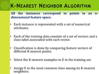
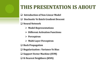
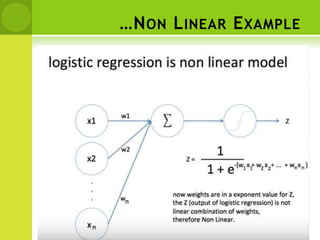
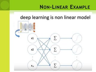
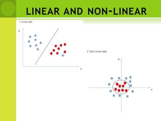
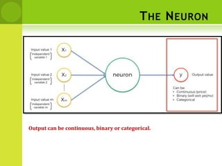
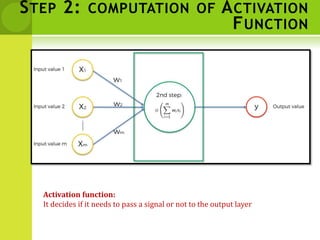
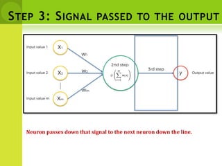
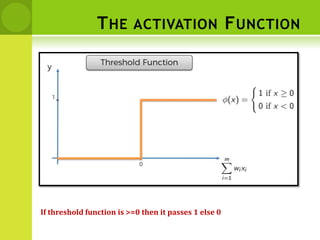
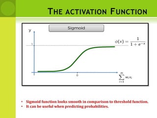
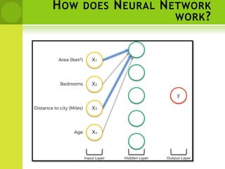
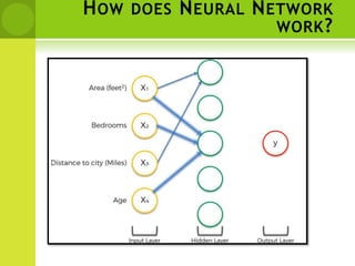
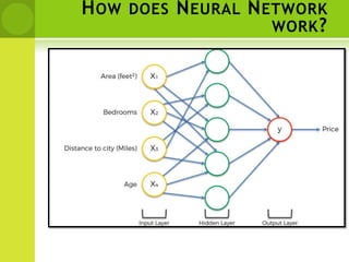
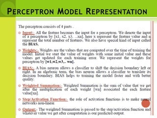
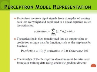
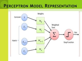
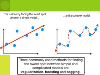
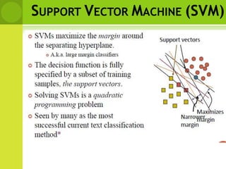
This document provides an overview of non-linear machine learning models. It introduces non-linear models and compares them to linear models. It discusses stochastic gradient descent and batch gradient descent optimization algorithms. It also covers neural networks, including model representations, activation functions, perceptrons, multi-layer perceptrons, and backpropagation. Additionally, it discusses regularization techniques to reduce overfitting, support vector machines, and K-nearest neighbors algorithms.

1. MACHINE LEARNING
MODULE 3
NON-LINEAR LEARNING

2.  Introduction of Non-Linear Model
 Stochastic Vs Batch Gradient Descent
 Neural Network
 Model Representations
 Different Activation Functions
 Perceptron
 Multi Layer Perceptron
 Back Propagation
 Regularization : Variance Vs Bias
 Support Vector Machine (SVM)
 K-Nearest Neighbors (KNN)
THIS PRESENTATION IS ABOUT

3. INTRODUCTION OF NON-LINEAR
MODEL

4. LINEAR MODEL
As long as we have weights in Linear combinations
we call it linear model in machine learning.
Linear Model Examples

5. LINEAR MODEL EXAMPLE
Linear Model Example:

6. NON-LINEAR MODEL
Non Linear Model Examples

7. …NON LINEAR EXAMPLE

8. NON-LINEAR EXAMPLE

9. NON-LINEAR MODEL
Can Linear Model has Curve Shape?
Yes
Since, Linear means Linear Combinations of
Weights, NOT the Shape of the Function.

10. NON-LINEAR MODEL

11. NON-LINEAR MODEL

12. NON-LINEAR MODEL

13. NON-LINEAR MODEL

14. NON-LINEAR MODEL

15. LINEAR AND NON-LINEAR

16. • In this method one training sample (example) is passed through
the neural network at a time and the parameters (weights) of each
layer are updated with the computed gradient.
• So, at a time a single training sample is passed through the network
and its corresponding loss is computed. The parameters of all the
layers of the network are updated after every training sample.
• For example, if the training set contains 100 samples then the
parameters are updated 100 times that is one time after every
individual example is passed through the network.
STOCHASTIC GRADIENT DESCENT

17. 1. It is easier to fit into memory due to a single training sample being
processed by the network
2. It is computationally fast as only one sample is processed at a time
3. For larger datasets it can converge faster as it causes updates to the
parameters more frequently
4. Due to frequent updates the steps taken towards the minima of the loss
function have oscillations which can help getting out of local minimums
of the loss function (in case the computed position turns out to be the
local minimum)
1. Due to frequent updates the steps taken towards the minima are very noisy.
This can often lead the gradient descent into other directions.
2. Also, due to noisy steps it may take longer to achieve convergence to the
minima of the loss function
3. Frequent updates are computationally expensive due to using all resources
for processing one training sample at a time
4. It loses the advantage of vectorized operations as it deals with only a single
example at a time
DISADVANTAGES OF STOCHASTIC GRADIENT DESCENT
ADVANTAGES OF STOCHASTIC GRADIENT DESCENT

18. BATCH GRADIENT DESCENT
• The concept of carrying out gradient descent is the same as
stochastic gradient descent. The difference is that instead of
updating the parameters of the network after computing the loss of
every training sample in the training set, the parameters are
updated once that is after all the training examples have been
passed through the network.
• For example, if the training dataset contains 100 training examples
then the parameters of the neural network are updated once.

19. ADVANTAGES OF BATCH GRADIENT DESCENT
1. Less oscillations and noisy steps taken towards the global minima of the
loss function due to updating the parameters by computing the average of
all the training samples rather than the value of a single sample
2. It can benefit from the vectorization which increases the speed of
processing all training samples together
3. It produces a more stable gradient descent convergence and stable error
gradient than stochastic gradient descent
4. It is computationally efficient as all computer resources are not being used
to process a single sample rather are being used for all training samples.
DISADVANTAGES OF BATCH GRADIENT DESCENT
1. Sometimes a stable error gradient can lead to a local minima and unlike
stochastic gradient descent no noisy steps are there to help get out of the
local minima.
2. The entire training set can be too large to process in the memory due to
which additional memory might be needed.
3. Depending on computer resources it can take too long for processing all
the training samples as a batch.

20. MINI BATCH GRADIENT DESCENT BATCH :
A COMPROMISE
• This is a mixture of both stochastic and batch gradient descent. The training
set is divided into multiple groups called batches. Each batch has a number
of training samples in it.
• At a time a single batch is passed through the network which computes the
loss of every sample in the batch and uses their average to update the
parameters of the neural network.
• For example, say the training set has 100 training examples which is divided
into 5 batches with each batch containing 20 training examples. This means
that the equation will be iterated over 5 times (number of batches).
This ensures the following advantages of both stochastic and batch
gradient descent are used due to which Mini Batch Gradient Descent is most
commonly used in practice.
1. Easily fits in the memory
2. It is computationally efficient
3. Benefit from vectorization
4. If stuck in local minimums, some noisy steps can lead the way out of them
5. Average of the training samples produces stable error gradients and
convergence.

21. NOISE IN GRADIENT DESCENT

22. NEURAL NETWORK

23. WHAT ARE NEURAL NETWORKS?
 Neural Networks are networks of neurons, for example, as
found in real (i.e. biological) brains
 Artificial neurons are crude approximations of the neurons
found in real brains. They may be physical devices, or purely
mathematical constructs.
 Artificial Neural Networks (ANNs) are networks of Artificial
Neurons and hence constitute crude approximations to parts
of real brains. They maybe physical devices, or simulated on
conventional computers.
 From a practical point of view, an ANN is just a parallel
computational system consisting of many simple processing
elements connected together in a specific way in order to
perform a particular task

24. ADVANTAGES
 They are extremely powerful computational devices.
 Massive parallelism makes them very efficient.
 They can learn and generalize from training data – so
there is no need for enormous feats of programming.
 They are particularly fault tolerant.
 They are very noise tolerant – so they can cope with
situations where normal symbolic systems would have
difficulty
 In principle, they can do anything a symbolic/logic
system can do, and more.

25. BOOLEAN FUNCTIONS AND PERCEPTRON

26. TYPES OF NEURAL NETWORK

27. TYPES OF NEURAL NETWORKS

28. THE NERVOUS SYSTEM

29. THE NEURON
• Dendrites receives the signals for the neuron.
• Axon transmits the signal from the neuron.
• Dendrites are connected to axon of the other neuron.
Signals from 1 neuron passes down to the next
neuron via axon
.

30. THE NEURON
Input layer is showing all the independent variable for one observation.

31. THE NEURON
Output can be continuous, binary or categorical.

32. THE NEURON
If it is categorical then
we might get multiple
outputs in terms of
dummy variables.
Eg: x1= age, x2= salary, xm = name Y= yes/ no
Will purchase a car?

33. THE NEURON
• Weights are adjusted by the process of learning
• It decides the importance/ strength of each signal
• Training a Neural network is based on Adjusting Weights

34. STEP 1: COMPUTATION OF WEIGHTED SUM OF
INPUT VALUES
Weighted sum of all Input Values

35. STEP 2: COMPUTATION OF ACTIVATION
FUNCTION
Activation function:
It decides if it needs to pass a signal or not to the output layer

36. STEP 3: SIGNAL PASSED TO THE OUTPUT
Neuron passes down that signal to the next neuron down the line.

37. THE ACTIVATION FUNCTION
If threshold function is >=0 then it passes 1 else 0

38. THE ACTIVATION FUNCTION
• Sigmoid function looks smooth in comparison to threshold function.
• It can be useful when predicting probabilities.

39. THE ACTIVATION FUNCTION

40. THE ACTIVATION FUNCTION

41. BRAIN TEASER
Assuming that your dependent variable is binary, what activation function
will you use?

42. BRAIN TEASER : ANSWER

43. PRACTICAL APPLICATION

44. May apply a rectifier function in
the hidden layer
Sigmoid function on
output layer

45. HOW DOES NEURAL NETWORK
WORK?

46. HOW DOES NEURAL NETWORK
WORK?

47. HOW DOES NEURAL NETWORK
WORK?

48. HOW DOES NEURAL NETWORK
WORK?

49. HOW DOES NEURAL NETWORK
WORK?

50. HOW NEURAL NETWORK LEARN
 Goal is to create a network that learns on its own.
 How can you distinguish cat and dog???
 Can learn on its own.

51. HOW NEURAL NETWORK LEARN

52. HOW NEURAL NETWORK LEARN

53. HOW NEURAL NETWORK LEARN
Cost function C tells the error

54. HOW NEURAL NETWORK LEARN
We update the weight in order to reduce cost function

55. HOW NEURAL NETWORK LEARN

56. PERCEPTRON

57. PERCEPTRON

58. …PERCEPETRON

59. PERCEPTRON MODEL REPRESENTATION

60. PERCEPTRON MODEL REPRESENTATION

61. PERCEPTRON MODEL REPRESENTATION

62. DIFFERENT ACTIVATION FUNCTIONS

63. MODEL REPRESENTATION:
EXAMPLE

64. DIFFERENT ACTIVATION FUNCTIONS

65. PERCEPTRON NODE – THRESHOLD
LOGIC UNIT
x1
xn
x2
w1
w2
wn
z
q
q
q
<
=
³
å
å
=
=
i
n
i
i
i
n
i
i
w
x
z
w
x
1
1
if
0
if
1
𝜽
• Learn weights such that an
objective function is maximized.
• What objective function should we
use?
• What learning algorithm should we
use?

66. PERCEPTRON LEARNING ALGORITHM
x1
x2
z
q
q
<
=
³
å
å
=
=
i
n
i
i
i
n
i
i
w
x
z
w
x
1
1
if
0
if
1
0.4
-0.2
0.1
x1 x2 t
0
1
.1
.3
.4
.8

67. FIRST TRAINING INSTANCE
q
q
<
=
³
å
å
=
=
i
n
i
i
i
n
i
i
w
x
z
w
x
1
1
if
0
if
1
0.8
0.3
z
0.4
-0.2
0.1
net = .8*.4 + .3*(-0.2) = 0.26
=1
x1 x2 t
0
1
.1
.3
.4
.8

68. SECOND TRAINING INSTANCE
q
q
<
=
³
å
å
=
=
i
n
i
i
i
n
i
i
w
x
z
w
x
1
1
if
0
if
1
x1 x2 t
0
1
.1
.3
.4
.8
.4
.1
z
.4
-.2
.01
net = .4*.4 + .1*-.2 = 0.14
=1
* c
Dwi = (t - z) * xi

69. SECOND EXAMPLE

70. PERCEPTRON RULE LEARNING
where wi is the weight from input i to perceptron node,
c is the learning rate,
t is the target for the current instance,
z is the current output,
xi is ith input
Dwi = (t - z)*c*xi
• Least perturbation principle
• Only change weights if there is an error
• small c rather than changing weights sufficient to make current
pattern correct
• Scale by xi
• Create a perceptron node with n inputs
• Iteratively apply a pattern from the training set and apply the
perceptron rule
• Each iteration through the training set is an epoch
• Continue training until total training set error ceases to improve
• Perceptron Convergence Theorem: Guaranteed to find a solution
in finite time if a solution exists

71. THE EXCLUSIVE OR PROBELM

72. THE XOR PROBELM

73. MULTI LAYER PERCEPTRON

74. MULTI LAYER PERCEPTRON

75. BACKPROPOGATION

76. BACKPROPOGATION: BASIC STEPS

77. BACKPROPOGATION

78. STEP1: FORWARD PASS

79. 79
FORWARD PASS

80. STEP2: BACKWARD PASS

81. BACKWARD PASS

83. STEP3: UPDATION OF WEIGHTS

84. …UPDATION OF WEIGHTS

85. SOLVED BACK PROPOGATION

91. Rough Work

93. VARIANCE VS BIAS

94. If no bias weight then
the hyperplane must
go through the origin
VARIATION VS BIAS

105. In Training Phase

108. What is Bias?
Bias is the difference between the average prediction of our model and
the correct value which we are trying to predict. Model with high bias
pays very little attention to the training data and oversimplifies the
model. It always leads to high error on training and test data.
What is Variance?
Variance is the variability of model prediction for a given data point or a
value which tells us spread of our data. Model with high variance pays a
lot of attention to training data and does not generalize on the data
which it hasn’t seen before. As a result, such models perform very well
on training data but has high error rates on test data.
BIAS AND VARIANCE

109. If our model is too simple and has very few parameters then it may
have high bias and low variance. On the other hand if our model
has large number of parameters then it’s going to have high
variance and low bias. So we need to find the right/good balance
without overfitting and underfitting the data.
Total Error = Bias^ 2 + Variance + Irreducible Error
WHY IS BIAS VARIANCE TRADEOFF?
An optimal balance of bias and
variance would never overfit or
underfit the model.

110. SUPPORT VECTOR MACHINE
https://www.youtube.com/watch?v=efR1C6CvhmE&t=255s
https://www.youtube.com/watch?v=Toet3EiSFcM&t=7s
https://www.youtube.com/watch?v=Qc5IyLW_hns&t=52s
Reference Links:

111. INTRODUCTION

112. SUPPORT VECTOR MACHINES

113. HYPERPLANE AS DECISION SURFACE

114. SUPPORT VECTORS

115. MAXIMIZING THE MARGIN

116. SUPPORT VECTOR MACHINE (SVM)

117. MAXIMUM MARGIN : FORMALIZATION

118. GEOMETRIC MARGIN

119. LINEAR SUPPORT VECTOR MACHINE

120. LINEAR SVM: THE LINEARLY SEPARABLE CASE

121. NON-LINEAR SVM

122. NON-LINEAR SVM: FEATURE SPACE

123. KERNELS

124. K-NEAREST NEIGHBOR

125. Simple Analogy..
• Tell me about your friends(who your neighbors
are) and I will tell you who you are.

126. Instance-based Learning
Its very similar to
a Desktop!!

127. KNN – DIFFERENT NAMES
127
• K-Nearest Neighbors
• Memory-Based Reasoning
• Example-Based Reasoning
• Instance-Based Learning
• Lazy Learning

128. WHAT IS KNN?
• A powerful classification algorithm used in pattern
recognition.
• K nearest neighbors stores all available cases and
classifies new cases based on a similarity
measure(e.g distance function)
• One of the top data mining algorithms used today.
• A non-parametric lazy learning algorithm (An
Instance-based Learning method).

129. KNN: CLASSIFICATION APPROACH
• An object (a new instance) is classified by a
majority votes for its neighbor classes.
• The object is assigned to the most common
class amongst its K nearest neighbors
(measured by a distant function ).

130. DISTANCE MEASURE
Training
Records
Test
Record
Compute
Distance
Choose k of the
“nearest” records

131. DISTANCE FUNCTIONS FOR CONTINUOUS VARIABLES

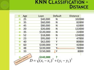
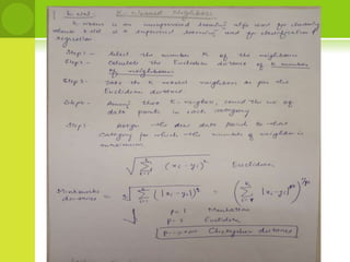
132. DISTANCE BETWEEN NEIGHBORS
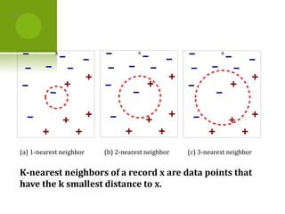
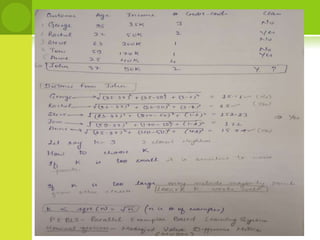
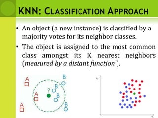
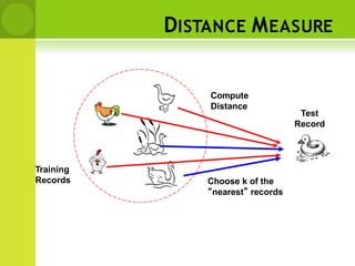
• Calculate the distance between new example
(E) and all examples in the training set.
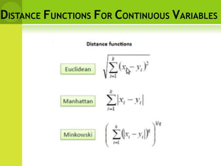
• Euclidean distance between two examples.
– X = [x1,x2,x3,..,xn]
– Y = [y1,y2,y3,...,yn]
– The Euclidean distance between X and Y is defined as
n
D(X ,Y)  (xi  yi )
i1
2

133. K-NEAREST NEIGHBOR ALGORITHM
• Each instance is represented with a set of numerical
attributes.
• Each of the training data consists of a set of vectors and a
class label associated with each vector.
• Classification is done by comparing feature vectors of
different K nearest points.
• Select the K-nearest examples to E in the training set.
• Assign E to the most common class among its K-nearest
neighbors.
All the instances correspond to points in an n-
dimensional feature space.

134. 3-KNN: EXAMPLE(1)

135. HOW TO SELECT K?
• If K is too small it is sensitive to noise points.
• Larger K works well. But too large K may include
majority points from other classes.
• Rule of thumb is K < sqrt(n), n is number of examples.
X

136. 136

137. X X X
(a) 1-nearest neighbor (b) 2-nearest neighbor (c) 3-nearest neighbor
K-nearest neighbors of a record x are data points that
have the k smallest distance to x.
137

138. KNN FEATURE
WEIGHTING
• Scale each feature by its importance for
classification.
• Can use our prior knowledge about which features
are more important
• Can learn the weights wk using cross‐validation

139. FEATURE NORMALIZATION
• Distance between neighbors could be dominated
by some attributes with relatively large
numbers.
e.g., income of customers in our previous example.
• Arises when two features are in different scales.
• Important to normalize those features.
– Mapping values to numbers between 0 – 1.

140. NOMINAL/CATEGORICAL DATA
• Distance works naturally with numerical attributes.
• Binary value categorical data attributes can be regarded
as 1 or 0.

141. KNN CLASSIFICATION
$50,000
$0
$100,000
$250,000
$200,000
$150,000
0 10 20 30 40 50 60 70
Non-Default
Default
Age
Loan$
20

142. KNN CLASSIFICATION –
DISTANCE
 Age Loan Default Distance
 25 $40,000 N 102000
 35 $60,000 N 82000
 45 $80,000 N 62000
 20 $20,000 N 122000
 35 $120,000 N 22000
 52 $18,000 N 124000
 23 $95,000 Y 47000
 40 $62,000 Y 80000
 60 $100,000 Y 42000
 48 $220,000 Y 78000
 33 $150,000 Y 8000
 48 $142,000 ?
2 2
2
1 2 1  y )
D  (x  x )  (y
142

143. KNN CLASSIFICATION –
STANDARDIZED DISTANCE
Distance
0.7652
0.5200
0.3160
0.9245
0.3428
0.6220
0.6669
0.4437
0.3650
0.3861
0.3771

X  Min
Max  Min
X s
143
Age Loan Default
0.125 0.11 N
0.375 0.21 N
0.625 0.31 N
0 0.01 N
0.375 0.50 N
0.8 0.00 N
0.075 0.38 Y
0.5 0.22 Y
1 0.41 Y
0.7 1.00 Y
0.325 0.65 Y
0.7 0.61 ?

144. STRENGTHS OF KNN
• Very simple and intuitive.
• Can be applied to the data from any distribution.
• Good classification if the number of samples is large enough.
Weaknesses of KNN
• Takes more time to classify a new example.
 need to calculate and compare distance from new
example to all other examples.
• Choosing k may be tricky.
• Need large number of samples for accuracy.

145. SOLVED K-NEAREST NEIGHBOR