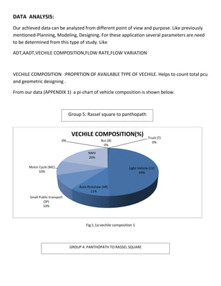
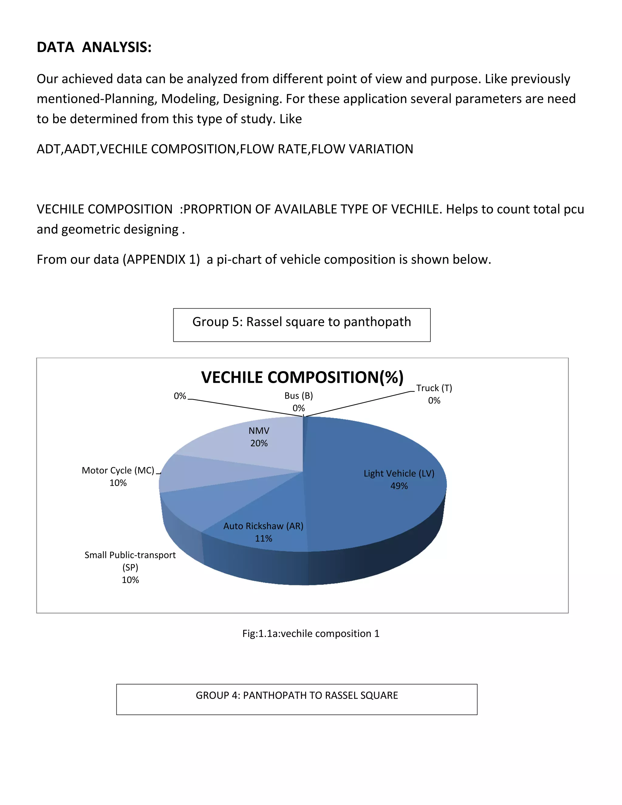
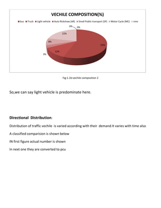
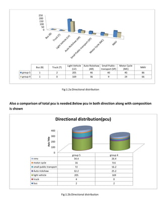
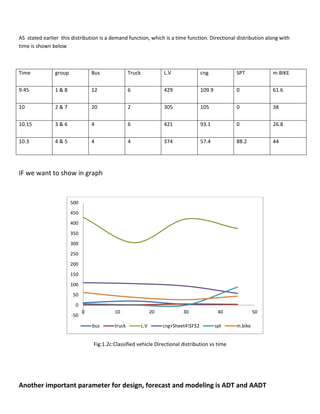
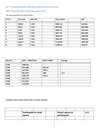
This document analyzes traffic data collected from two locations: Rassel Square to Panthopath and Panthopath to Rassel Square. The analysis includes: 1. Vehicle composition - Light vehicles make up 49% of traffic, while motorcycles and auto rickshaws each make up 10%. 2. Directional distribution - Traffic flows vary by time of day and direction. More vehicles travel from Panthopath to Rassel Square compared to the opposite direction. 3. Average daily traffic (ADT) and annual average daily traffic (AADT) - ADT and AADT are calculated for each location to understand typical and annual traffic volumes.

1. DATA ANALYSIS:
Our achieved data can be analyzed from different point of view and purpose. Like previously
mentioned-Planning, Modeling, Designing. For these application several parameters are need
to be determined from this type of study. Like
ADT,AADT,VECHILE COMPOSITION,FLOW RATE,FLOW VARIATION
VECHILE COMPOSITION :PROPRTION OF AVAILABLE TYPE OF VECHILE. Helps to count total pcu
and geometric designing .
From our data (APPENDIX 1) a pi-chart of vehicle composition is shown below.
Fig:1.1a:vechile composition 1
Bus (B)
0%
Truck (T)
0%
Light Vehicle (LV)
49%
Auto Rickshaw (AR)
11%
Small Public-transport
(SP)
10%
Motor Cycle (MC)
10%
NMV
20%
0%
VECHILE COMPOSITION(%)
Group 5: Rassel square to panthopath
GROUP 4: PANTHOPATH TO RASSEL SQUARE

2. Fig:1.1b:vechile composition 2
So,we can say light vehicle is predominate here.
Directional Distribution:
Distribution of traffic vechile is varied according with their demand.It varies with time also
A classified comparision is shown below
IN first figure actual number is shown
In next one they are converted to pcu
0% 0%
55%
12%
3%
8%
22%
VECHILE COMPOSITION(%)
bus Truck Light vehicle Auto Rickshaw (AR) Small Public-transport (SP) Motor Cycle (MC) nmv

3. Fig:1.2a:Directional distribution
Also a comparison of total pcu is needed.Below pcu in both direction along with composition
is shown
Fig:1.2b:Directional distribution
0
50
100
150
200
250
Bus (B) Truck (T)
Light Vehicle
(LV)
Auto Rickshaw
(AR)
Small Public-
transport (SP)
Motor Cycle
(MC)
NMV
group 5 1 2 205 46 40 40 86
group 4 1 0 169 36 9 24 66
0
100
200
300
400
group 5 group 4
nmv 34.4 26.4
motor cycle 16 9.6
small public transport 72 16.2
Auto rickshaw 32.2 25.2
light vehicle 205 169
truck 4 0
bus 2 2
AxisTitle
Directional distribution(pcu)

4. AS stated earlier this distribution is a demand function, which is a time function. Directional distribution along with
time is shown below
Time group Bus Truck L.V cng SPT m.BIKE
9.45 1 & 8 12 6 429 109.9 0 61.6
10 2 & 7 20 2 305 105 0 38
10.15 3 & 6 4 6 421 93.1 0 26.8
10.3 4 & 5 4 4 374 57.4 88.2 44
IF we want to show in graph
Fig:1.2c:Classified vehicle Directional distribution vs time
Another important parameter for design, forecast and modeling is ADT and AADT
-50
0
50
100
150
200
250
300
350
400
450
500
0 10 20 30 40 50
bus truck L.V cng+Sheet4!$F$2 spt m.bike

5. ADT : The equivalent hourly traffic flow measured in less than one hour
AADT: Total yearly volume divided by number of days
This two parameter are shown below
GROUP Flow rate EXP. FAC 7day volume ADT
1 1563.2 7.012 10961.16 1565.88
2 856.8 7.012 6007.882 858.2688
3 1430 7.012 10027.16 1432.451
4 993.6 7.012 6967.123 995.3033
5 1462.4 7.012 10254.35 1464.907
6 1064.8 7.012 7466.378 1066.625
7 1023.2 7.012 7174.678 1024.954
8 1610 7.012 11289.32 1612.76
Exp.FAC AADT 1 DIRECTION AADT 2 DIREC Average
0.948 1484.454
0.948 813.6388 3013.29
0.948 1357.964 1785.2
0.948 943.5475 2369 2375
0.948 1388.732 2332.2
0.948 1011.161
0.948 971.6564
0.948 1528.896
Another parameter flow rate is shown below-
Panthopath to rassel
square
Rassel square to
panthopath
total

6. total pcu 248.4 365.6 614
elapsed time 15 15 15
Flow
rate(pcu/day)
993.6 1462.4 2456
Flow fluctuation:
Travel demand varies with time,season ,weather .Urban and rural fluctuation has definite
pattern.
For our work fluctuation curve is like below

7. Fig 1.3a:flow fluctuation
In urban area two peaks should be there.But as we take a very short count it is not occurring here
0
100
200
300
400
500
600
700
800
900
0 5 10 15 20 25 30 35 40 45
Series1
Series2
Series3