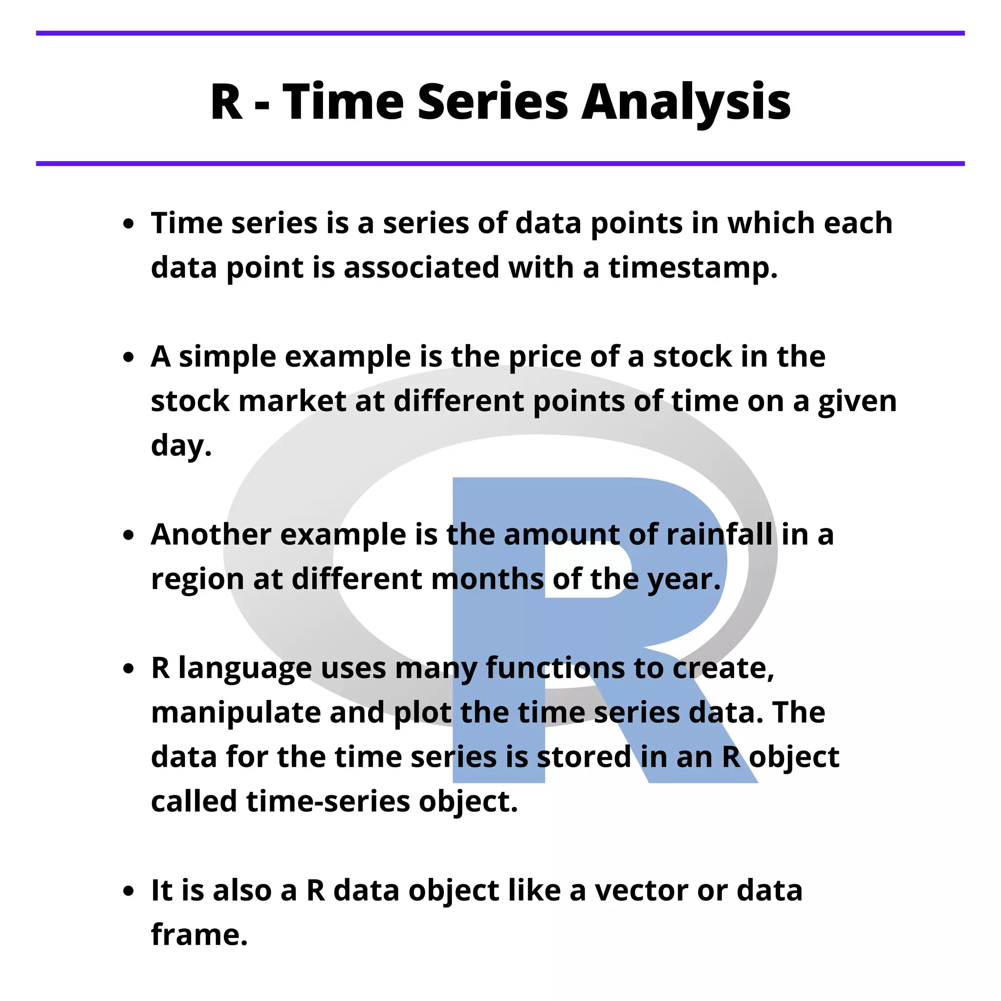
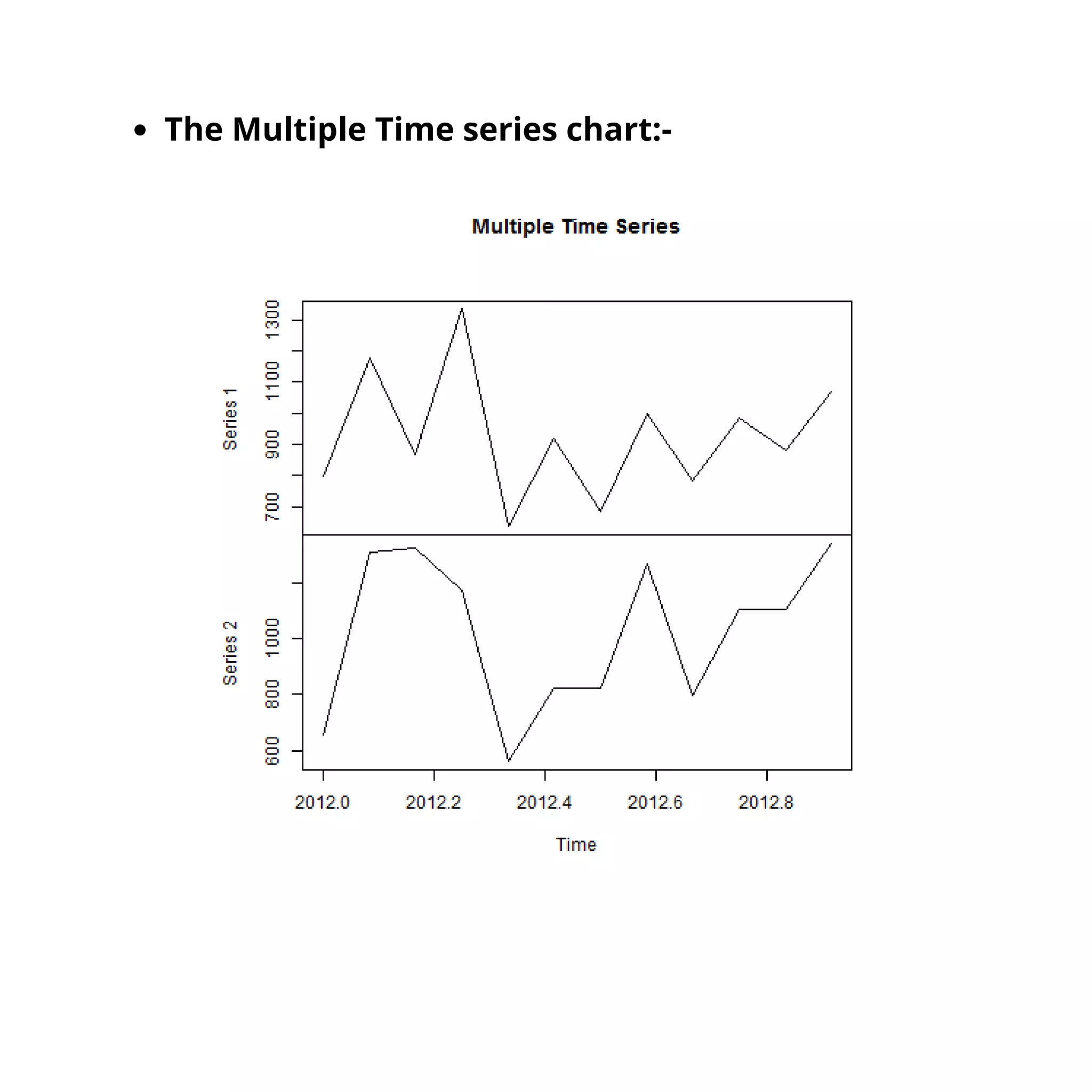
This document provides an overview of time series analysis using the R programming language, explaining how to create, manipulate, and plot time series data with the ts() function. It illustrates the creation of time series objects with examples like annual rainfall, and demonstrates how to combine multiple time series into a single chart. The document also details the significance of the frequency parameter in determining the time intervals for data points.

1. Swipe
R - Time Series Analysis

2. Time series is a series of data points in which each
data point is associated with a timestamp.
A simple example is the price of a stock in the
stock market at different points of time on a given
day.
Another example is the amount of rainfall in a
region at different months of the year.
R language uses many functions to create,
manipulate and plot the time series data. The
data for the time series is stored in an R object
called time-series object.
It is also a R data object like a vector or data
frame.
R - Time Series Analysis

3. The time series object is created by using the ts()
function.
The basic syntax for ts() function in time series
analysis is:-
timeseries.object.name <- ts(data, start, end,
frequency)
Following is the description of the parameters
used:-
data is a vector or matrix containing the values
used in the time series.
start specifies the start time for the first
observation in time series.
end specifies the end time for the last
observation in time series.
frequency specifies the number of
observations per unit time.

4. Example
Consider the annual rainfall details at a place
starting from January 2012. We create an R time
series object for a period of 12 months and plot it.
# Get the data points in form of a R vector.
rainfall <-
c(799,1174.8,865.1,1334.6,635.4,918.5,685.5,998.6,784.2,
985,882.8,1071)
# Convert it to a time series object.
rainfall.timeseries <- ts(rainfall,start =
c(2012,1),frequency = 12)
# Print the timeseries data.print(rainfall.timeseries)#
Give the chart file a name.
png(file = "rainfall.png")
# Plot a graph of the time series.
plot(rainfall.timeseries)
# Save the file.
dev.off()

5. When we execute the above code, it produces the
following result and chart:-
Jan Feb Mar Apr May Jun Jul Aug Sep
2012 799.0 1174.8 865.1 1334.6 635.4 918.5 685.5
998.6 784.2
Oct Nov Dec
2012 985.0 882.8 1071.0

6. The Time series chart:-

7. Different Time Intervals
The value of the frequency parameter in the ts()
function decides the time intervals at which the
data points are measured.
A value of 12 indicates that the time series is for
12 months. Other values and its meaning is as
below:-
frequency = 12 pegs the data points for every
month of a year.
frequency = 4 pegs the data points for every
quarter of a year.
frequency = 6 pegs the data points for every 10
minutes of an hour.
frequency = 24*6 pegs the data points for every
10 minutes of a day.

8. Multiple Time Series
We can plot multiple time series in one chart by
combining both the series into a matrix.
# Get the data points in form of a R vector.
rainfall1 <-
c(799,1174.8,865.1,1334.6,635.4,918.5,685.5,998.6,784.2,985,882.
8,1071)
rainfall2 <-
c(655,1306.9,1323.4,1172.2,562.2,824,822.4,1265.5,799.6,1105.6,
1106.7,1337.8)
# Convert them to a matrix.
combined.rainfall <- matrix(c(rainfall1,rainfall2),nrow = 12)
# Convert it to a time series object.
rainfall.timeseries <- ts(combined.rainfall,start =
c(2012,1),frequency = 12)

9. # Print the timeseries data.print(rainfall.timeseries)
# Give the chart file a name.
png(file = "rainfall_combined.png")
# Plot a graph of the time series.
plot(rainfall.timeseries, main = "Multiple Time
Series")
# Save the file.
dev.off()

10. When we execute the above code, it produces the
following result and chart:-
Series 1 Series 2
Jan 2012 799.0 655.0
Feb 2012 1174.8 1306.9
Mar 2012 865.1 1323.4
Apr 2012 1334.6 1172.2
May 2012 635.4 562.2
Jun 2012 918.5 824.0
Jul 2012 685.5 822.4
Aug 2012 998.6 1265.5
Sep 2012 784.2 799.6
Oct 2012 985.0 1105.6
Nov 2012 882.8 1106.7
Dec 2012 1071.0 1337.8

11. The Multiple Time series chart:-

12. R - Nonlinear Least Square
R - Decision Tree
Tableau - Quick Guide
Stay Tuned with
Topics for next Post