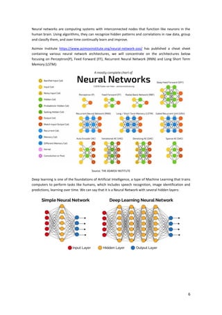
Download to read offline

![3
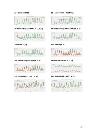
ARMA Algorithm
Auto Regressive Moving Average - ARMA is an autoregressive moving average model. It is simply the
fusion between the AR (p) and MA (q) models. The AR(p) model attempts to explain the timing and
average reversal effects frequently observed in markets (market participant effects). The MA(q) model
attempts to capture the observed shock effects in terms of white noise. These shock effects can be
considered unexpected events that affect the observation process, p, such as sudden gains, wars,
attacks, etc.
The ARMA model tries to capture these two aspects when modeling time series, it does not take into
account volatility clustering, an empirical phenomenon essential to many financial time series.
O Modelo ARMA(1,1) é representado como: x(t) = ax(t-1) + be(t-1) + e(t), onde e(t) é o ruído branco com
E [e(t)] = 0.
The ARMA(1,1) Model is represented as: x(t) = ax(t-1) + be(t-1) + e(t), where e(t) is white noise with
E [e(t)] = 0.
An ARMA model generally requires fewer parameters than an AR(p) model or an individual MA(q)
model.
ARIMA Algorithm
Autoregressive Integrated Moving Average - ARIMA is an autoregressive integrated moving average
model, a generalization of an ARMA model.
Both models are fitted to time series data to better understand the data or to predict future points in
the series (forecast). ARIMA models are applied in some cases where the data show evidence of non-
stationarity, where an initial differentiation step (corresponding to the "integrated" part of the model)
can be applied one or more times to eliminate non-stationarity.
The AR part of ARIMA indicates that the evolving variable of interest is regressed with its own lagged (ie,
prior) values. The I (for "integrated") indicates that the data values have been replaced by the difference
between their values and the previous values (and this differentiating process may have been
performed more than once). The goal of each of these features is to make the model fit the data as well
as possible. The MA part indicates that the regression error is actually a linear combination of error
terms whose values occurred contemporaneously and at various times in the past.
Non-seasonal ARIMA models are usually designated ARIMA(p, d, q), where the parameters p, d and q
are non-negative integers, p is the order (number of time intervals) of the autoregressive model, d is the
degree of differentiation (the number of times the data had past values subtracted) and q is the order of
the moving average model.
SARIMAX Algorithm
Seasonal Autoregressive Integrated Moving Average - SARIMAX is a seasonal autoregressive integrated
moving average model with the parameters (p, d, q) (P, D, Q) m, where m refers to the number of
periods in each seasonality and the capital letters P, D, Q refer to the autoregressive, differentiated, and
moving average terms of the seasonal part of the ARIMA model.](https://image.slidesharecdn.com/socialdistancingdistimeseries-220514160209-9603fce9/85/Social_Distancing_DIS_Time_Series-3-320.jpg)
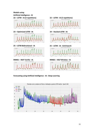

This article presents a strategy for population service in the fight against COVID-19 using a scenario simulator that incorporates artificial intelligence and system dynamics. It details the modeling of social distancing predictions through various statistical and machine learning algorithms and aims to enhance understanding of factors influencing disease transmission. Future work involves utilizing simulation results to create geospatial visualizations and further refine predictive modeling efforts.


