This document discusses time series forecasting using the ARIMA model in Python. It begins with an overview of forecasting and time series analysis. It then covers the key components of time series like trends, seasonality and randomness. Next, it explains techniques like simple average, exponential smoothing, ARMA and ARIMA models. Finally, it provides the major steps for time series forecasting using ARIMA in Python, including importing packages, decomposing the time series, checking stationarity, identifying p,q,d values, training and testing the model, making predictions and evaluating the model.

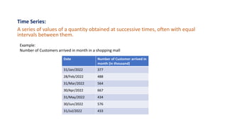
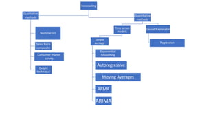
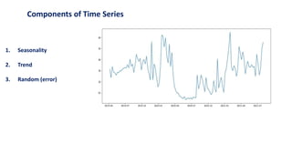
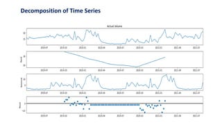
1. Time Series Forecasting:
ARIMA Model Using Python

2. • Utility of the topic
• Forecasting
• Time Series
• Techniques of Forecasting
• Time Series and its Components
• Time series models: ARMA and ARIMA
• Steps and coding in python

3. • Industrial Utility
Provide Forecasts for decision making, such as
future price of stocks based on the past prices
Number of complaints
Demand for a product
Customer arrival
• Academic Utility
Data Analytics part of Operations and Supply Chain Management
MDP can be developed
Provides help in learning more decision making models
Python provides the foundation for digital transformation of operations

4. • Forecasting is the process of estimating a future event by casting
forward past data
• It assumes that future is the function of past
• Forecasting is a vital function and affects every significant
management decision
For example :
• Finance and accounting use forecasts as the basis for budgeting
and cost control
• Marketing relies on forecasts to make key decisions such as new
product planning and personnel compensation
• Production uses forecasts to select suppliers; determine
capacity requirements; and drive decisions about purchasing,
staffing, and inventory

5. Time Series:
A series of values of a quantity obtained at successive times, often with equal
intervals between them.
Date Number of Customer arrived in
month (in thousand)
31/Jan/2022 377
28/Feb/2022 488
31/Mar/2022 564
30/Apr/2022 667
31/May/2022 434
30/Jun/2022 576
31/Jul/2022 433
Example:
Number of Customers arrived in month in a shopping mall

6. Forecasting
Qualitative
methods
Nominal GD
Sales force
composite
Consumer market
survey
Delphi
technique
Quantitative
methods
Time series
models
Simple
average
Exponential
Smoothing
Autoregressive
Moving Averages
ARMA
ARIMA
Causal/Explanator
Regression

7. Components of Time Series
1. Seasonality
2. Trend
3. Random (error)

8. Decomposition of Time Series

9. 1. Simple Average
• Depends on the detecting the central tendency of demand
January February March April May June
200 250 260 280 270 290
Example,
Consider the Tata Sky monthly new connections in a city are as follows:
Forecast, the demand for July month

10. 2. Exponential Smoothing
Ft= F(t−1) + α[D(t−1)- F(t−1)] ------------------------- (1)
Where,
F= Forecast
𝛼 = Smoothing coefficient (0≤ 𝛼 ≤ 1)
D = Demand
t = is the period
t-1 = immediate previous period.
Expanding the exponential form, the equivalent form of equation (1) becomes,
Ft=α(1−α)0 D (t−1) + α(1−α)1 D(t−2) + α(1−α)2 D(t−3)

11. 3. Autoregressive Models (AR Model)
forecast the variable of interest using a linear combination of past values of the variable. The
term autoregression indicates that it is a regression of the variable against itself.
Y(t)=c+ϕ1y(t−1)+ϕ2y(t−2)+⋯+ϕpy(t−p)+ε(t)
Rather than using past values of the forecast variable in a regression, a moving average model uses past
forecast errors in a regression-like model.
Y(t)=c+ε(t)+θ1ε(t−1)+θ2ε(t−2)+⋯+θqε(t−q)
4. Moving Average Models (MA Model)
5. ARMA model
AR + MA

12. 6. ARIMA Model
Autoregressive Integrated Moving Average Model
ARMA + Differencing = ARIMA (p,d,q)
If we combine differencing with autoregression and a moving average model, we obtain a non-seasonal ARIMA model.

13. Forecasting with ARIMA in Python
Important Codes:
import pandas as pd
import numpy as np
import matplotlib.pylab as plt
from statsmodels.tsa.seasonal import seasonal_decompose
from statsmodels.tsa.stattools import adfuller, acf, pacf
from statsmodels.tsa.stattools import arma_order_select_ic
from statsmodels.graphics.tsaplots import plot_acf,plot_pacf
from statsmodels.tsa.arima.model import ARIMA
from sklearn.metrics import mean_squared_error
from datetime import datetime
df['Date']=pd.to_datetime(df['Date'])
indexed_df=df.set_index(df['Date'])
ts=indexed_df['Actuals']
ts.head()
plt.plot(ts)
decompose=seasonal_decompose(ts_am)
fig=decompose.plot()
Major Steps
Step 1: install packages
numpy, pandas, matplotlib
Step 2: from statsmodels.tsa import
Decompose, MSE, ADfuller, ACF, PACF, ARIMA
Step 3: covert data to time series
Step 4: plot and decompose time series

14. Forecasting with ARIMA in Python
Important Codes:
adftest=adfuller(timeseries)
print('pvalue of adfuller test is:', adftest[1])
plot_acf(ts_am)
plot_pacf(ts_am)
predict=model.predict(start=len(train),end=len (ts_w)-1)
error=np.sqrt(mean_squared_error(test,predict))
train.plot(legend=True, label ='train')
test.plot(legend=True, label ='test')
predict.plot(legend=True, label ='prediction ARIMA’)
final_model=ARIMA(ts_w,order=(1,0,2)).fit()
forecast=final_model.predict(len(ts_w),len(ts_w)+6)
ts_w.plot(legend=True,label='train')
forecast.plot(legend=True, label='forecast')
Major Steps
Step 5: Stationarity Check
Adfuller test
Step 6: finding p,q,d
ACF and PACF plots
Step 7: Test and Train Split
Step 8: predict values Using ARIMA model
Step 9: validity of model
Step 10: find the Forecast

15. Thank you