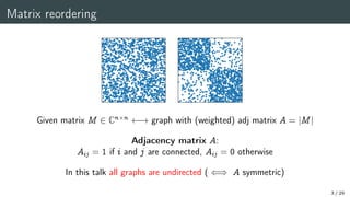
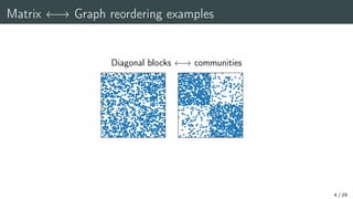
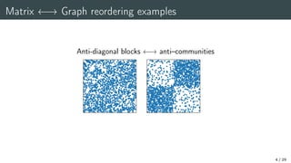
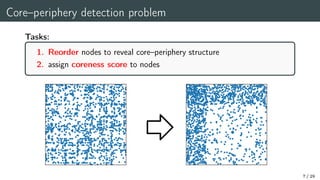
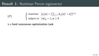
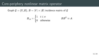
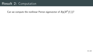
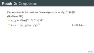
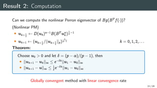
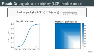
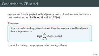
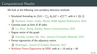
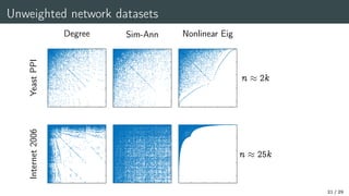
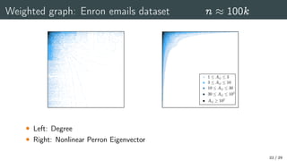
The document presents research on optimal L-shaped matrix reordering for core-periphery detection in networks, exploring tasks like reordering nodes and assigning core scores. It discusses the formulation of a core-periphery kernel optimization problem, nonlinear Perron eigenvector calculations, and convergence methods. The results emphasize computational approaches for core-periphery detection and analyze various methods and their effectiveness using real-world datasets.

1. Optimal L-shaped matrix reordering,
a.k.a. graph’s core-periphery
Francesco Tudisco
Gran Sasso Science Institute (Italy)
CIRM Luminy – NMSC2021
Numerical Methods and Scientific Computing
1 / 29

2. Thanks to
Des Higham
(Edinburgh, UK)
T, Higham, A nonlinear spectral method for core-periphery detection in
networks, SIAM J. Mathematics of Data Science, 2019
2 / 29

3. Matrix reordering
3 / 29

4. Matrix reordering
Given matrix M 2 Cnn ! graph with (weighted) adj matrix A = jMj
Adjacency matrix A:
Aij = 1 if i and j are connected, Aij = 0 otherwise
In this talk all graphs are undirected ( () A symmetric)
3 / 29

5. Matrix ! Graph reordering examples
Diagonal blocks ! communities
4 / 29

6. Matrix ! Graph reordering examples
Anti-diagonal blocks ! anti–communities
4 / 29

7. Matrix ! Graph reordering examples
Banded ! small–world
4 / 29

8. Matrix ! Graph reordering examples
L-shaped ! core–periphery
4 / 29

9. Graph visualization
5 / 29

10. Core–periphery in networks
Borgatti, Everett, Social Networks, 1999
Core: nodes strongly
connected across the
whole network
Periphery: nodes
strongly connected
only to the core
6 / 29

11. Core–periphery detection problem
Tasks:
1. Reorder nodes to reveal core–periphery structure
2. assign coreness score to nodes
7 / 29

12. Core–periphery kernel optimization
Core–score vector u is such that :
if ui uj =
) i is closer to the core than j
Our proposal:
Core–score vector as solution of the following constrained core–periphery
kernel optimization
(P)
8
:
maximize f(u) =
Pn
i;j=1 Aij(ui;uj)
subject to kukp = 1;u 0
with (x;y) =
x+y
2
1=
8 / 29

13. Core-periphery kernel
large ) (x;y) maxfx;yg
f(u) =
P
ij Aij(ui;uj) is large when
edges Aij = 1 involve at least one node
with large core-score
9 / 29

14. Connection with node degrees
If p = 2 and = 1 then 1 = arithmetic mean
(P) () max
u0
kAuk1
kuk2
= kAk2!1
and the maximizer is
u = degree vector
10 / 29

15. Connection with eigenvector centrality
If p = 1 and = 0 then 0 = geometric mean
(P) () max
u0
uT Au
uT u
= (A)
and the maximizer is
u = Perron eigenvector of A
What about the general case?
11 / 29

16. Main results
12 / 29

17. Result 1: Nonlinear Perron eigenvector
(P)
8
:
maximize f(u) =
Pn
i;j=1 Aij(u
i + u
j )1=
subject to kukp = 1;u 0
is a hard nonconvex optimization task
13 / 29

18. Result 1: Nonlinear Perron eigenvector
(P)
8
:
maximize f(u) =
Pn
i;j=1 Aij(u
i + u
j )1=
subject to kukp = 1;u 0
is a hard nonconvex optimization task
Theorem:
If 0 and p maxf1;g, then
(P) has a unique solution u
u is positive if and only if no zero rows in A
u is the nonlinear Perron eigvector of a “nonlinear matrix operator”
13 / 29

19. Core-periphery nonlinear matrix operator
Graph G = (V;E), B jV jjEj incidence matrix of G
Bi;e =
8
:
1 i 2 e
0 otherwise
BBT A
14 / 29

20. Core-periphery nonlinear matrix operator
Graph G = (V;E), B jV jjEj incidence matrix of G
Bi;e =
8
:
1 i 2 e
0 otherwise
BBT A
Nonlinear Perron eigenvector means
u 0 is the unique positive eigenvector solution to
Bg(BT f(x)) = x
with eigenvalue = maxfjj : solves that eigenvalue equationg
f;g are entrywise functions: g(x) = x1
1
and f(x) = x=(p )
14 / 29

21. Result 2: Computation
Can we compute the nonlinear Perron eigenvector of Bg(BT f())?
15 / 29

22. Result 2: Computation
Can we compute the nonlinear Perron eigenvector of Bg(BT f())?
(Nonlinear PM)
uk+ 1
2
D(uk) 1
B(BT u
k)
1
1
uk+1 (uk+ 1
2
=kuk+ 1
2
kp)
1
p 1 k = 0;1;2;:::
15 / 29

23. Result 2: Computation
Can we compute the nonlinear Perron eigenvector of Bg(BT f())?
(Nonlinear PM)
uk+ 1
2
D(uk) 1
B(BT u
k)
1
1
uk+1 (uk+ 1
2
=kuk+ 1
2
kp)
1
p 1 k = 0;1;2;:::
Theorem:
Choose u0 0 and let = (p )=(p 1), then
kuk+1 ukk1 e kku1 u0k1
kuk+1 uk1 1
e kku1 u0k1
Globally convergent method with linear convergence rate
15 / 29

24. Note on the analysis
We do not require that the objective function is convex. Instead, we use
the homogeneity f(x) = f(x) of the objective and the constraint
functions
Unlike communities, we can compute the a L-shaped reordering globally
optimally
We do not require the network to be connected (matrix to be irreducible)
in order to have uniqueness and positivity
16 / 29

25. Result 3: Logistic core–periphery (LCP) random model
Random graph G LCP(u) if Pr(i $ j) =
1
1 + e (ui;uj)
Logistic function
0.0 0.2 0.4 0.6 0.8 1.0
0.0
0.2
0.4
0.6
0.8
1.0
1/(1
−
e
−
x
)
x
Matrix of probabilities
0.1
0.2
0.3
0.4
0.5
0.6
0.7
0.8
0.9
17 / 29

26. Connection to CP kernel
Suppose we have a graph G with adjacency matrix A and we want to find a u
that maximizes the likelihood that G is LCP(u)
18 / 29

27. Connection to CP kernel
Suppose we have a graph G with adjacency matrix A and we want to find a u
that maximizes the likelihood that G is LCP(u)
Theorem:
If u is a node labeling (permutation), then the maximum likelihood prob-
lem is equivalent to
max
u
n
X
i;j=1
Aij(ui;uj)
(Useful for testing core–periphery detection algorithms)
18 / 29

28. How it behaves in practice
19 / 29

29. Computational Results
We look at the following core–periphery detection methods:
Simulated Annealing on f(x) =
P
ij Aij(x
i + x
j )1=, with x 2 f0;1g
Rombach, Porter, Fowler, Mucha SIAM Applied Mathematics, 2014
Coreness score as limit of H-index
Lu, Zhou, Zhang, Stanley, Nature communications, 2016
Degree vector of the graph
Csermely, London, Wu, Uzzi, Journal of Complex Networks, 2013
Perron eigenvector of the adjacency matrix
Mondragon, Journal of Complex Networks, 2017
Nonlinear Perron Eigenvector or NSM, with = 10 and p = 20
20 / 29

30. Unweighted network datasets
Degree Sim-Ann Nonlinear Eig
Yeast
PPI
n 2k
Internet
2006
n 25k
21 / 29

31. Weighted graph: Enron emails dataset n 100k
Left: Degree
Right: Nonlinear Perron Eigenvector
22 / 29

32. Core–periphery profiles
Persistance probability of the set S V : (V = set of all the nodes)
(S) =
P
i;j2S Aij
P
i2S
P
j2V Aij
Probability that a random walker who is currently in any of the nodes of S,
remains in S at the next time step
23 / 29

33. Core–periphery profiles
Sort the nodes by their (inverse) core-score:
Permutation 1;:::;n such that u1 u2 un
For any k = 1;:::;n consider Sk = f1;:::;kg and evaluate
(Sk)
24 / 29

34. Core–periphery profiles
0 500 1000 1500 2000
k
10−3
10−2
10−1
100
γ
k
(
x
)
Eig
Sim-Ann
Coreness
Deg
NSM
Yeast PPI
0 5000 10000 15000 20000
k
10−4
10−3
10−2
10−1
100
Eig
Sim-Ann
Coreness
Deg
NSM
Internet 2006
25 / 29

35. Objective function and LCP likelihood
NSM
Eig
Degree
Coreness
Sim-Ann
f(x) =
P
ij Aij(x
i + x
j )1=
Left: objective function f(x) evalued on differend core-score vectors
Right: log-likelihood when fitting a LCP random model
26 / 29

36. Top ten London train stations
= 0
Adjacency Eigenvector
= 10
Simulated Annealing
= 10
Nonlinear Perron Eigenvector
27 / 29

37. Top ten London train stations
Eigenvector Sim-Ann NSM
King’s Cross 128.85 Embankment 26.84 King’s Cross 128.85
Farringdon 29.75 King’s Cross 128.85 Baker Str. 29.75
Euston Square 14.40 Liverpool Str. 138.95 West Ham 77.10
Barbican 11.97 Baker Str. 29.75 Liverpool Str. 138.95
Gt Port. Str. 86.60 Bank 96.52 Paddington 85.32
Moorgate 38.40 Moorgate 38.40 Stratford 129.01
Euston 87.16 Euston Square 14.40 Embankment 26.84
Baker Str. 29.75 Gloucester Road 13.98 Willesden Junct. 109.27
Liverpool Str. 138.95 Farringdon 27.92 Moorgate 38.40
Angel 22.10 West Ham 77.10 Earls Court 20.00
Total 586.09 592.70 783.48
+35%
Data collected in: Cipolla, Durastante, T., Nonlocal PageRank
28 / 29

38. Thank you! Any question?
Best wishes to Claude Brezinski!
29 / 29