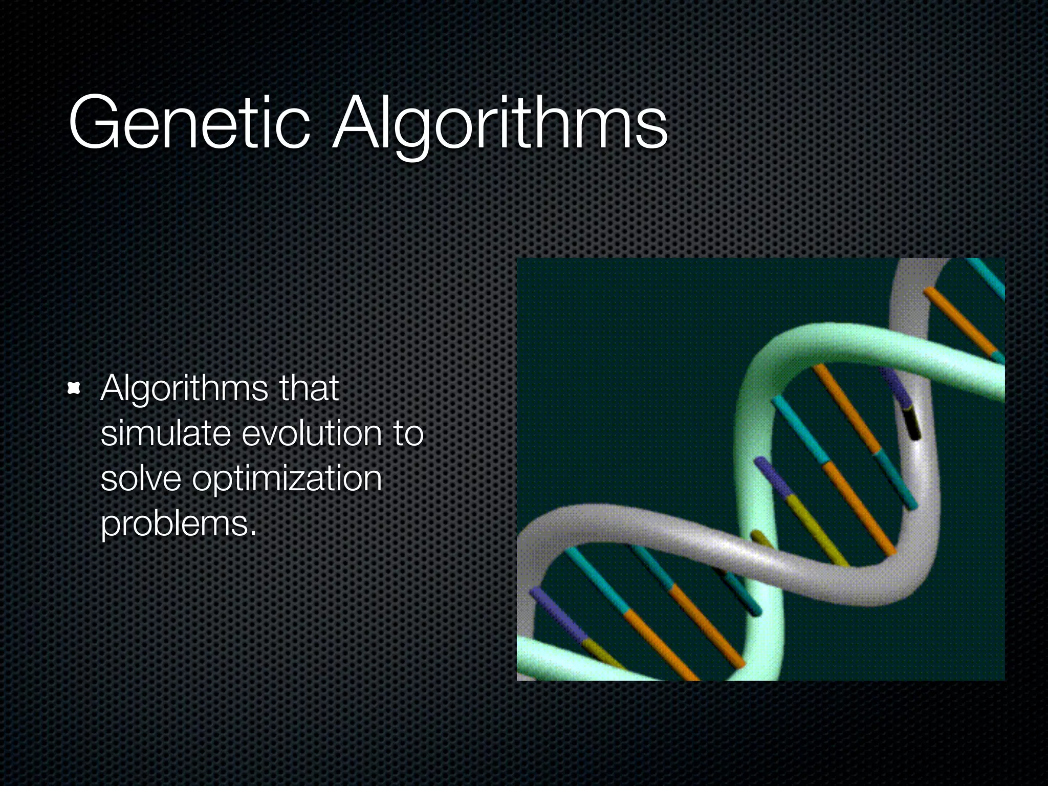
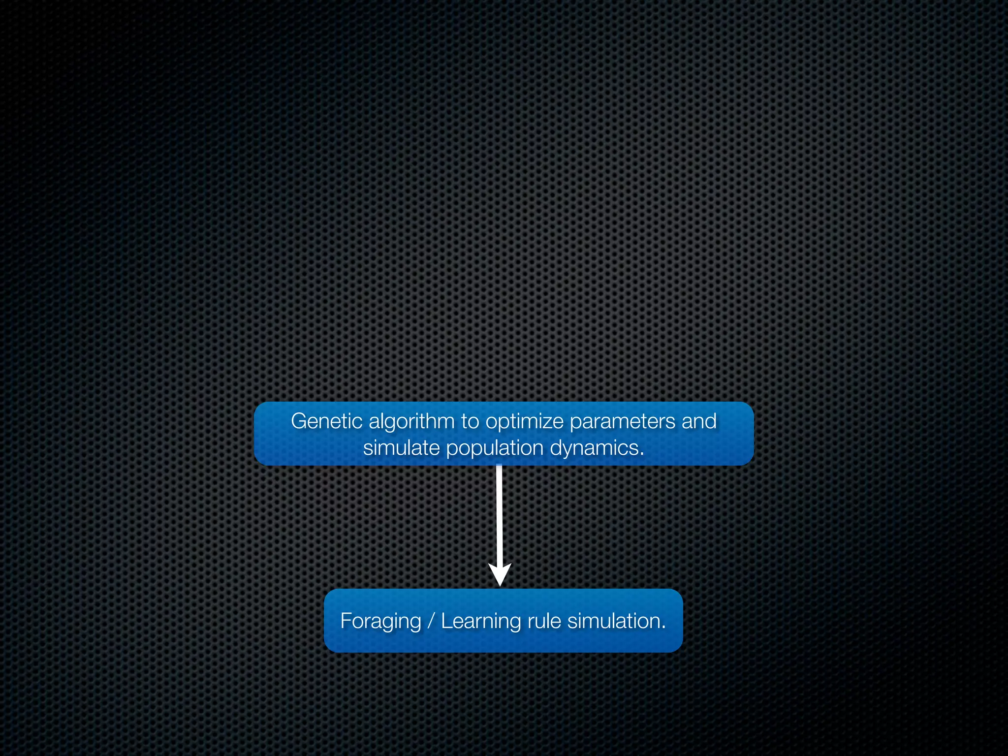
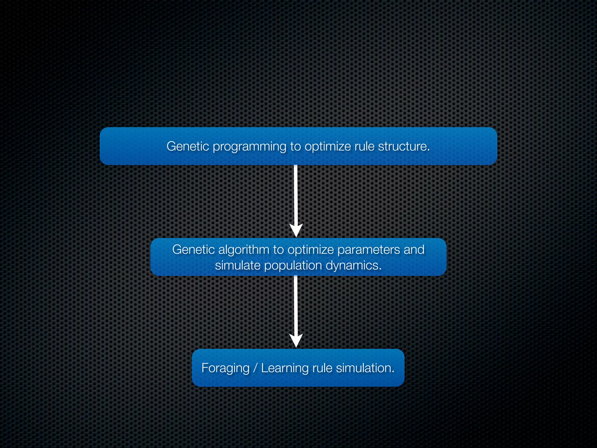
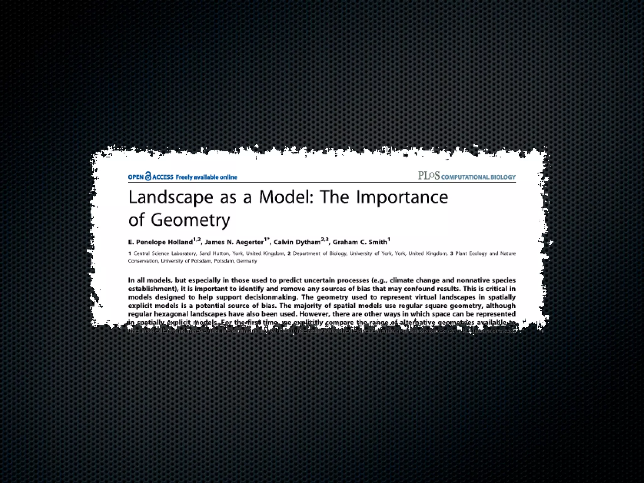
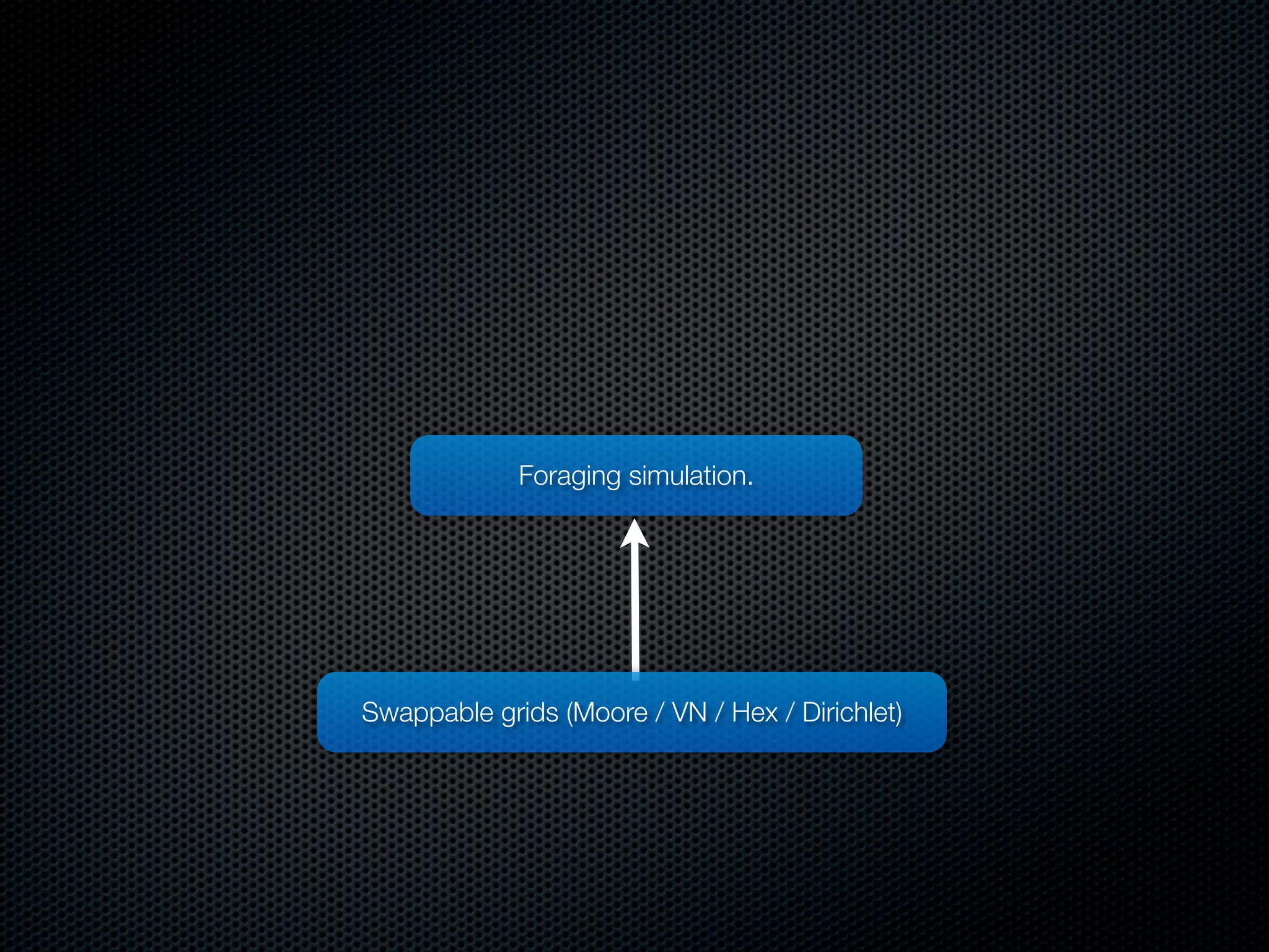
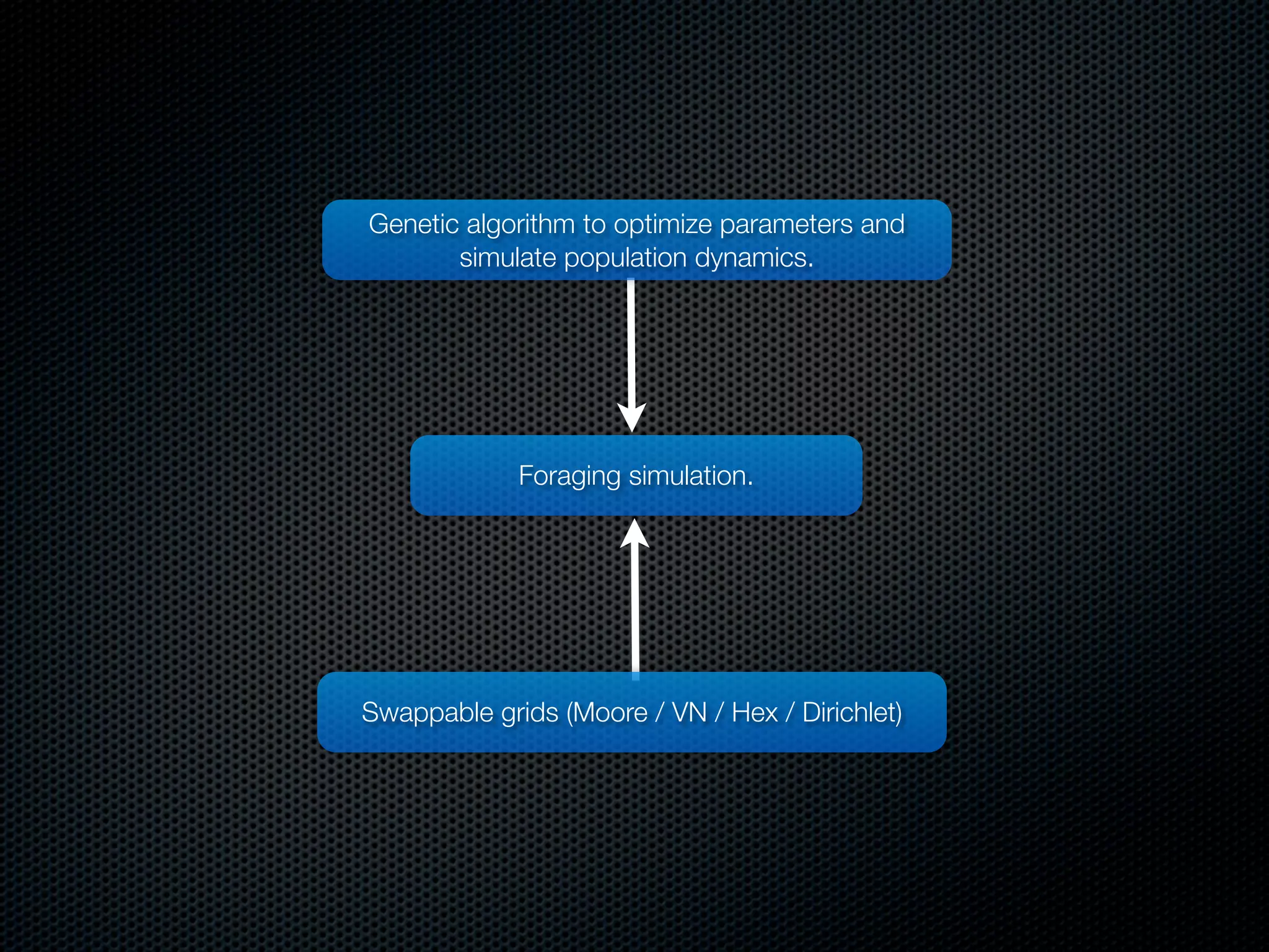
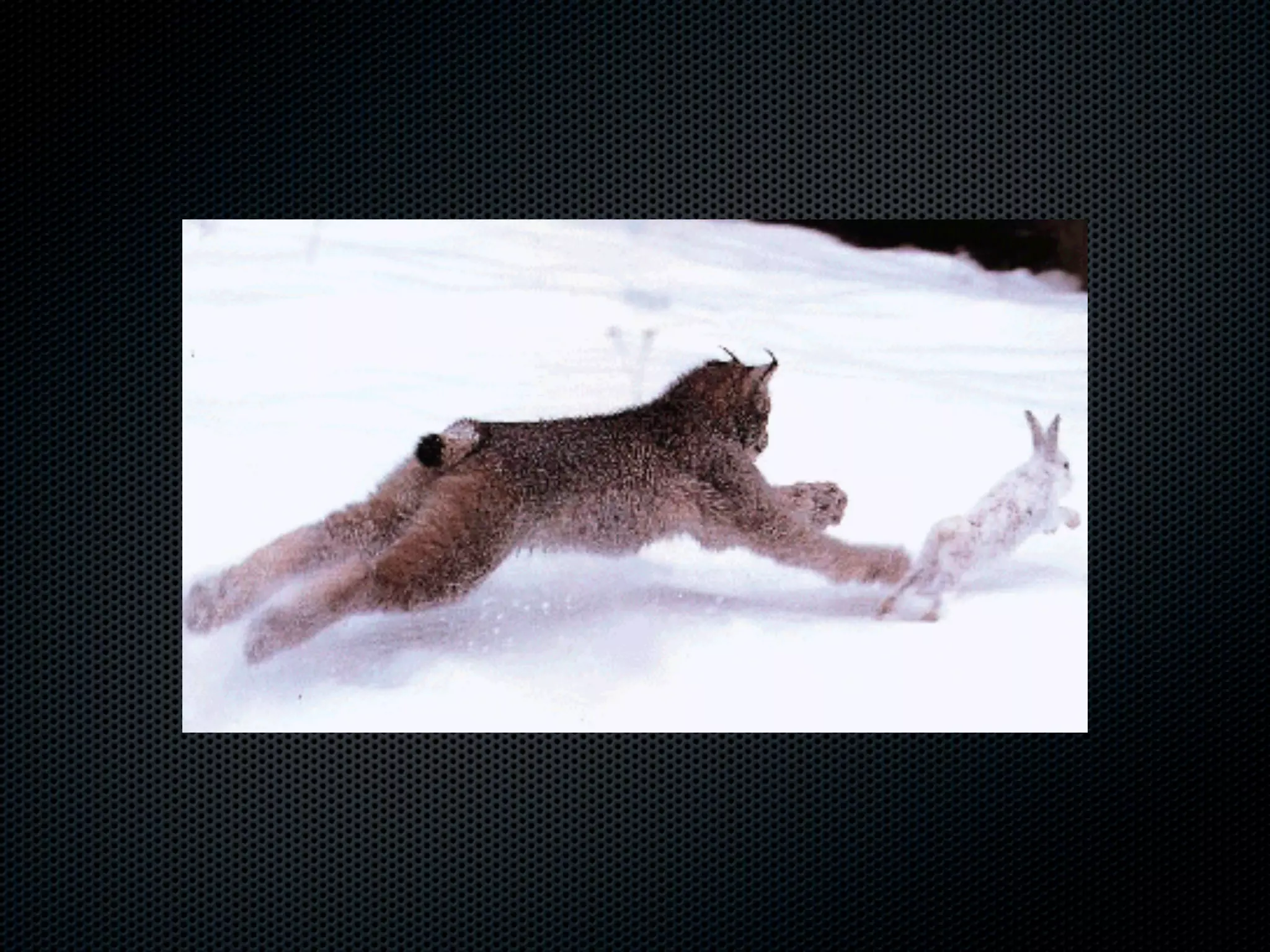
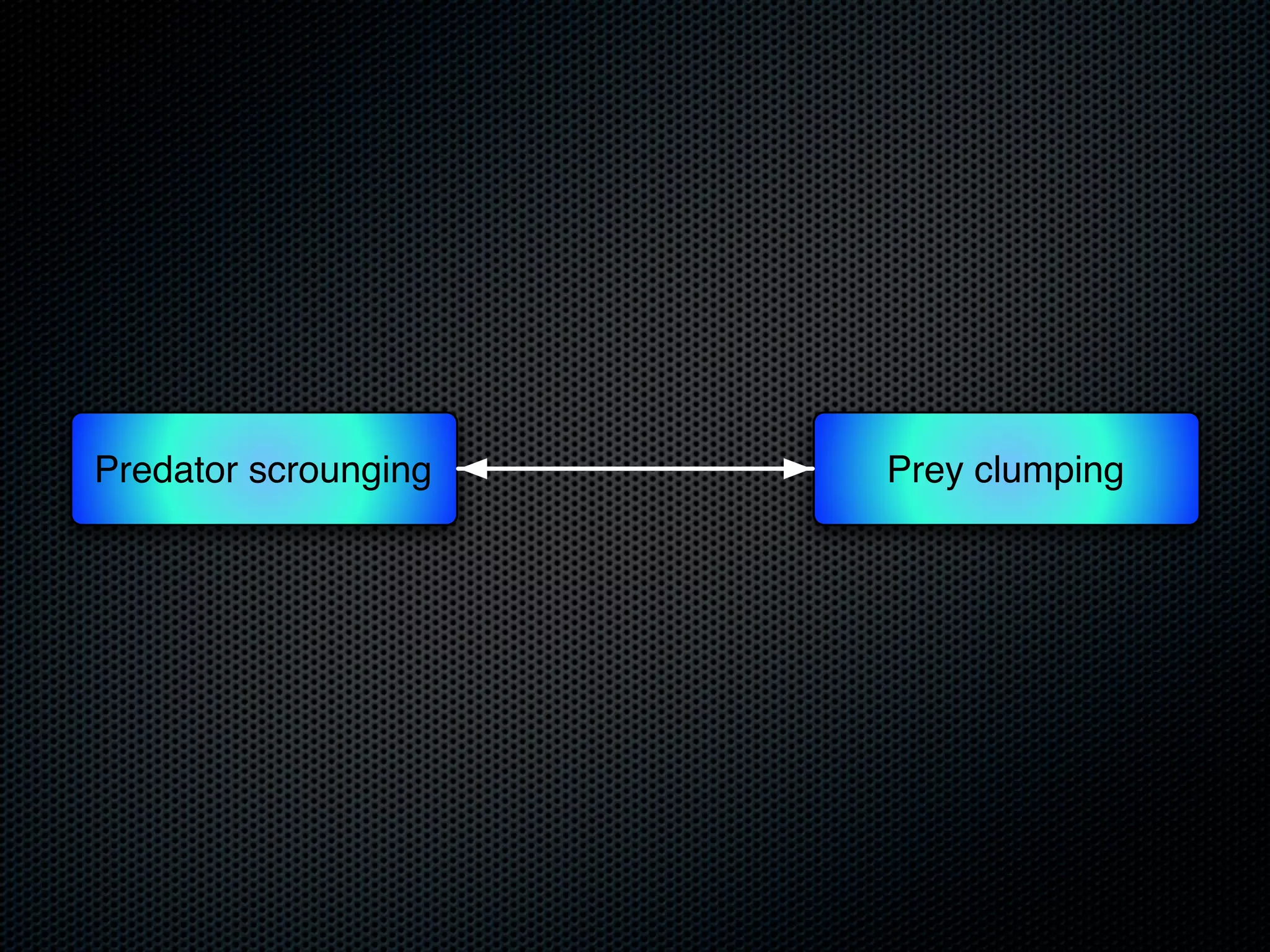
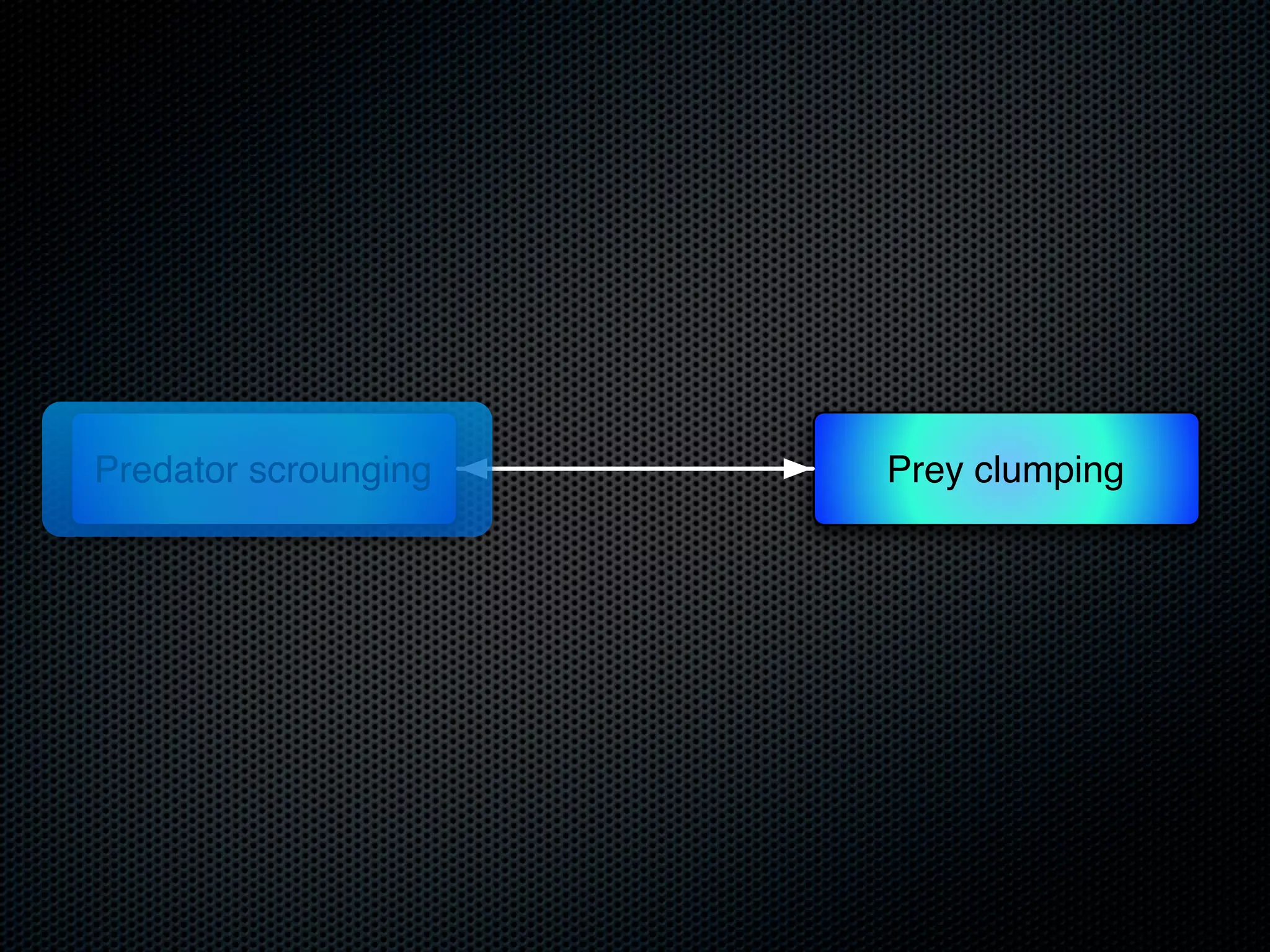
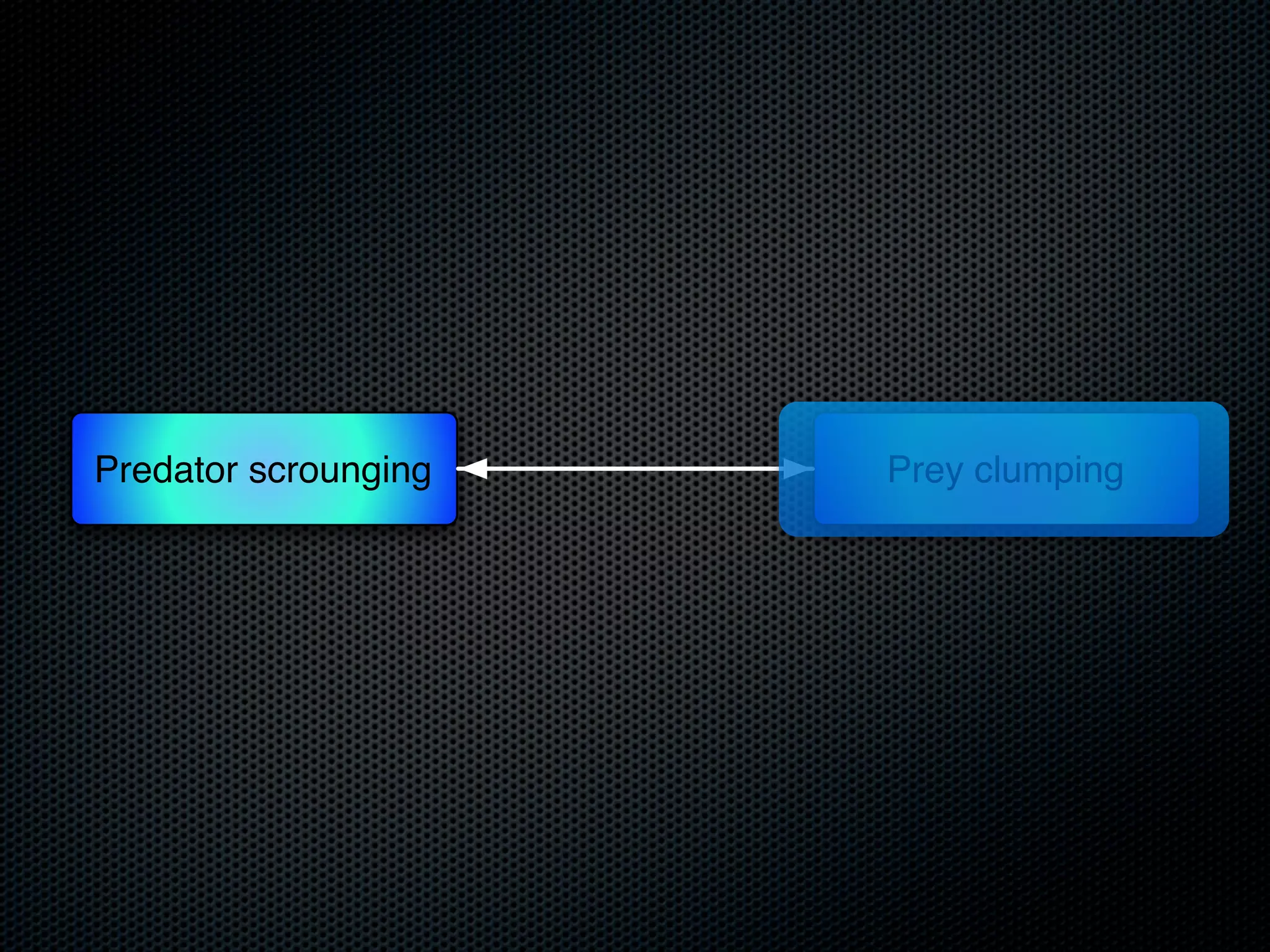
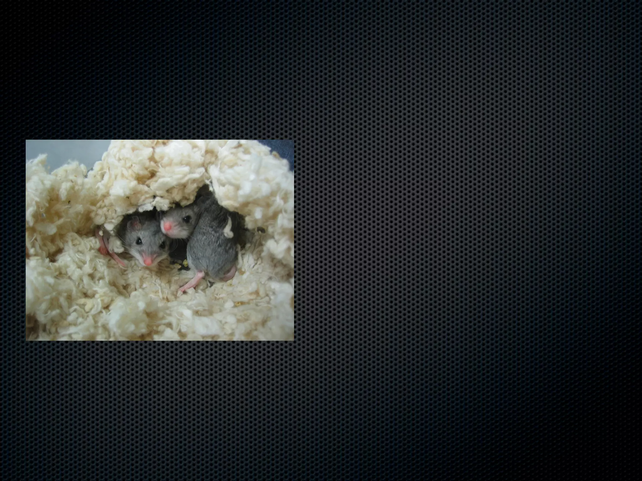
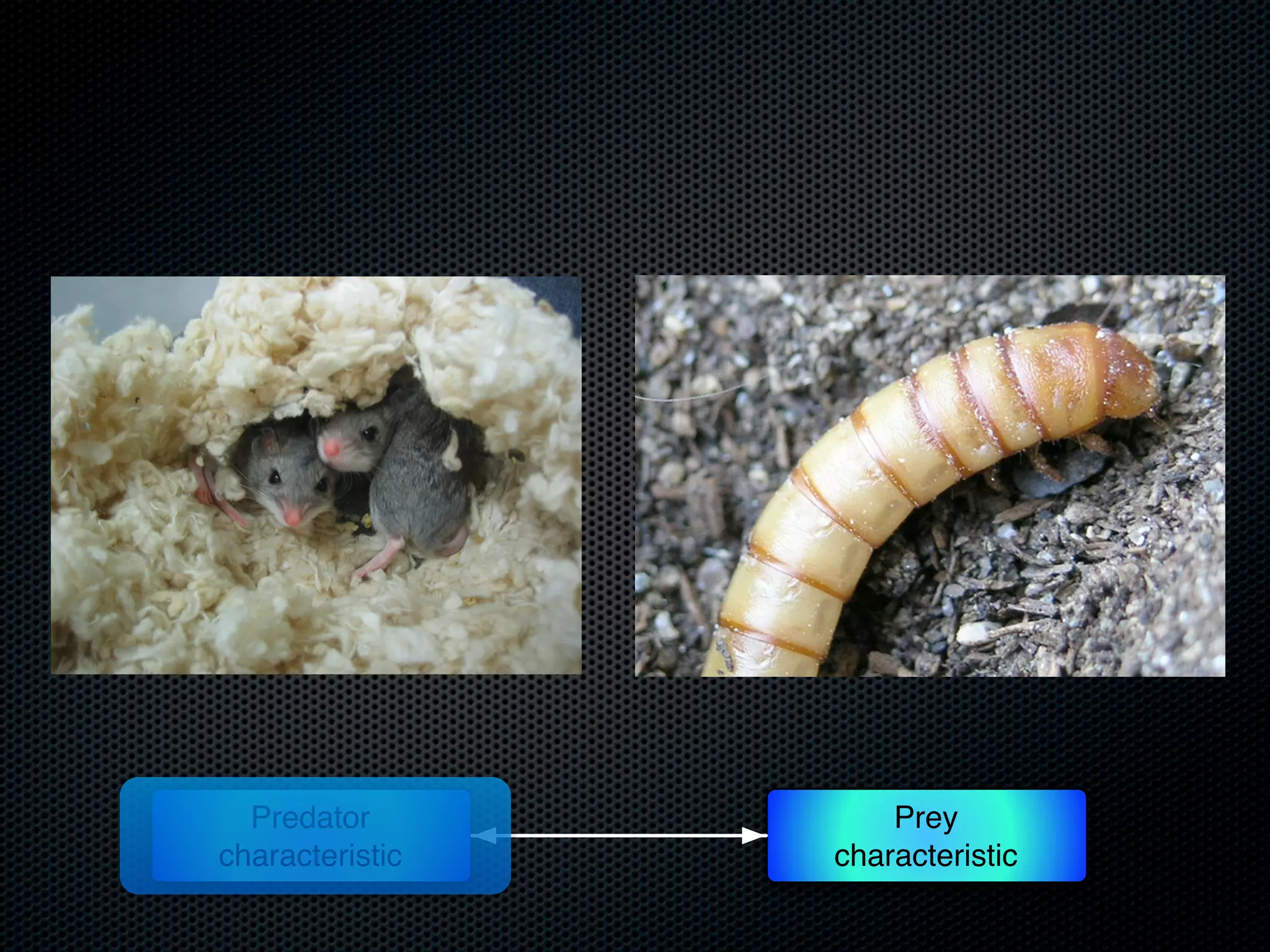
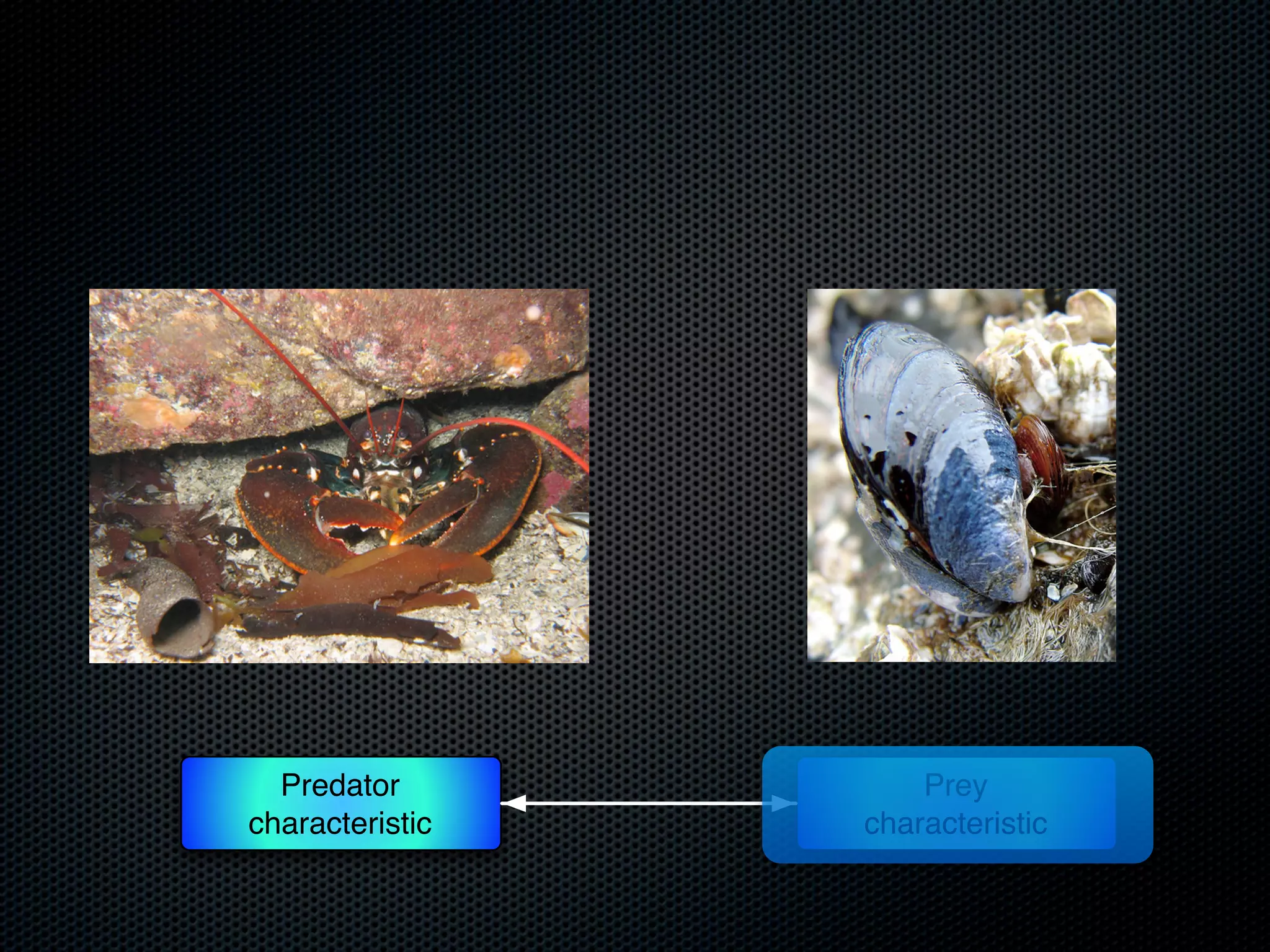
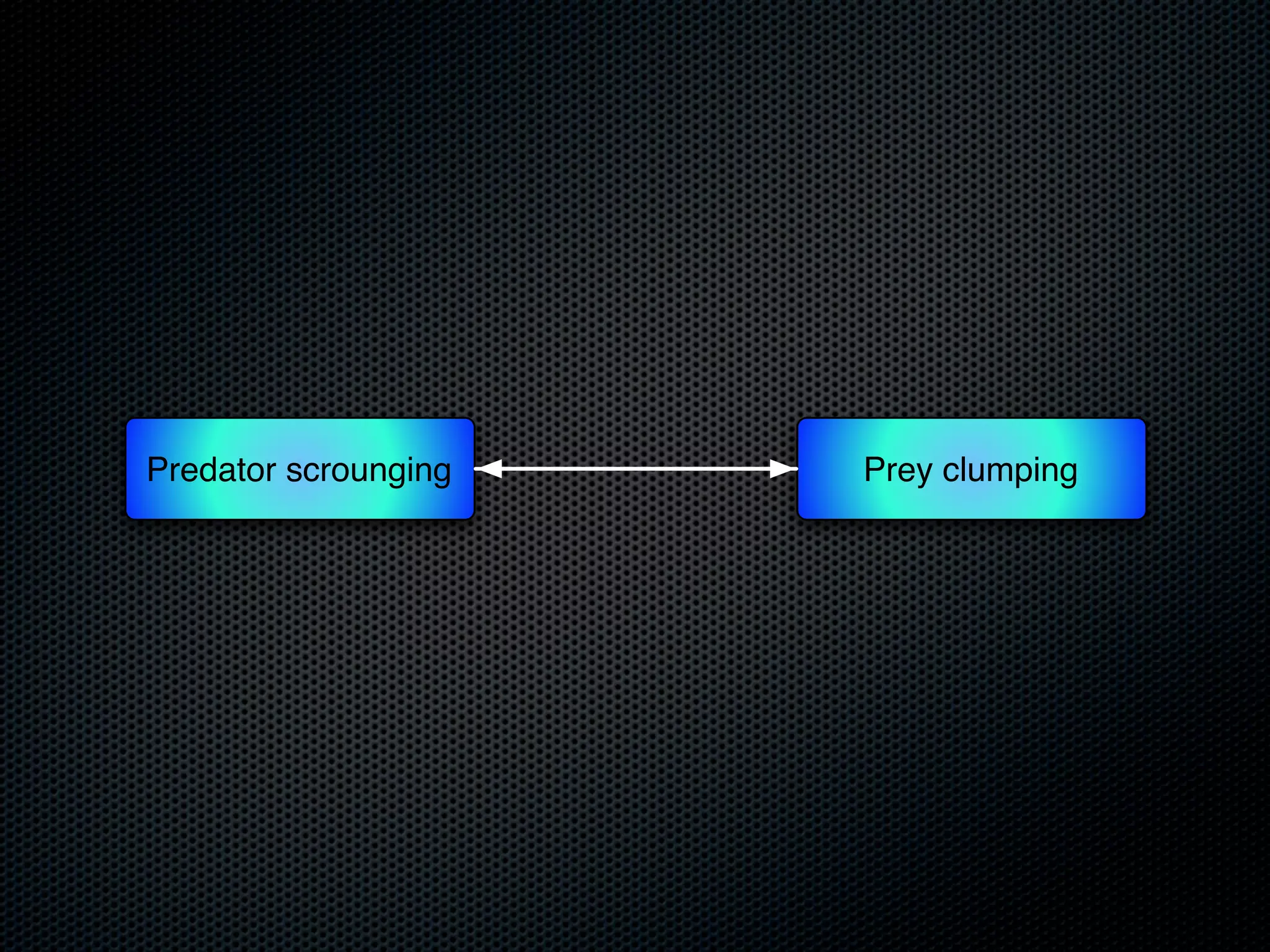
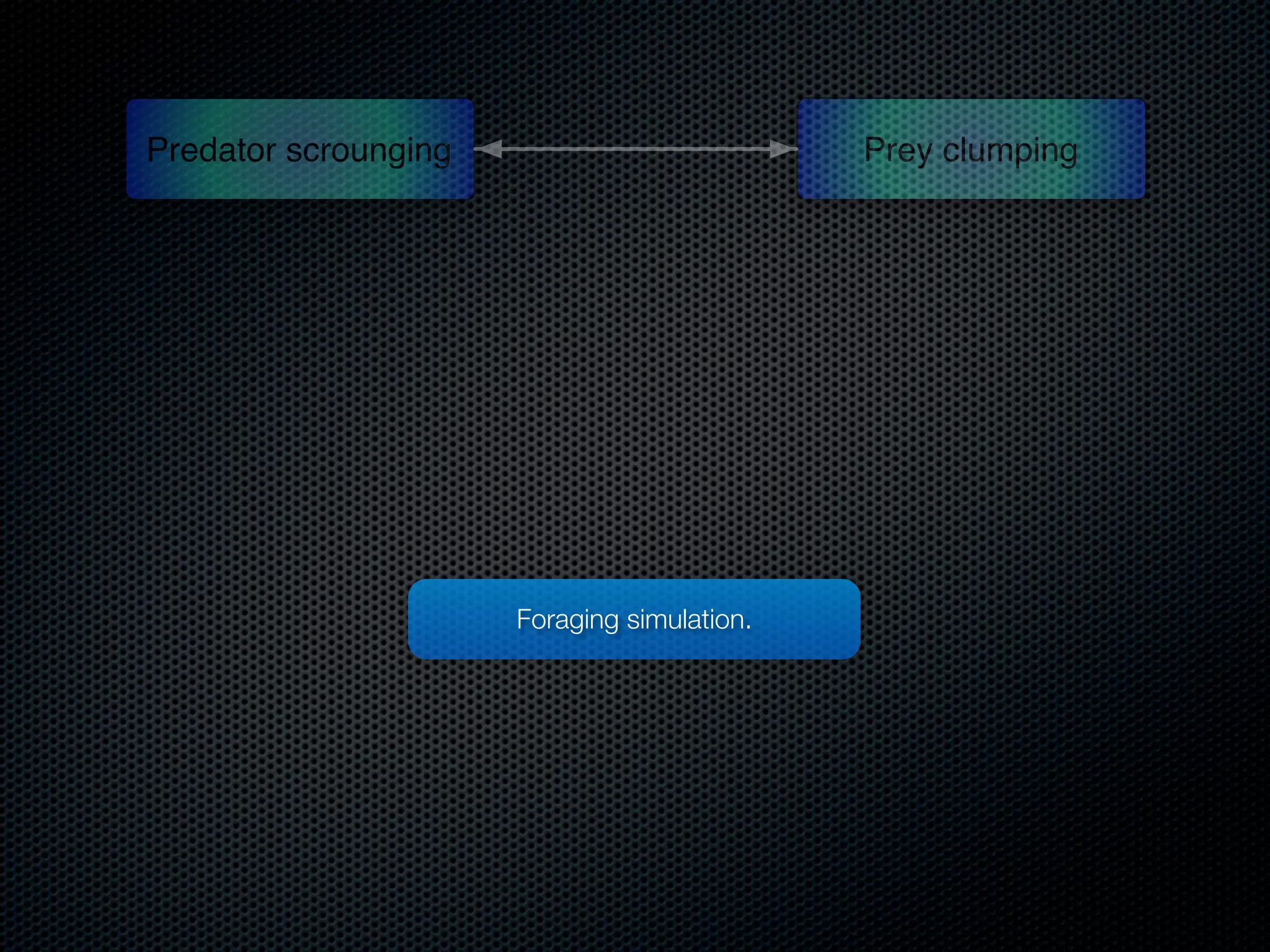
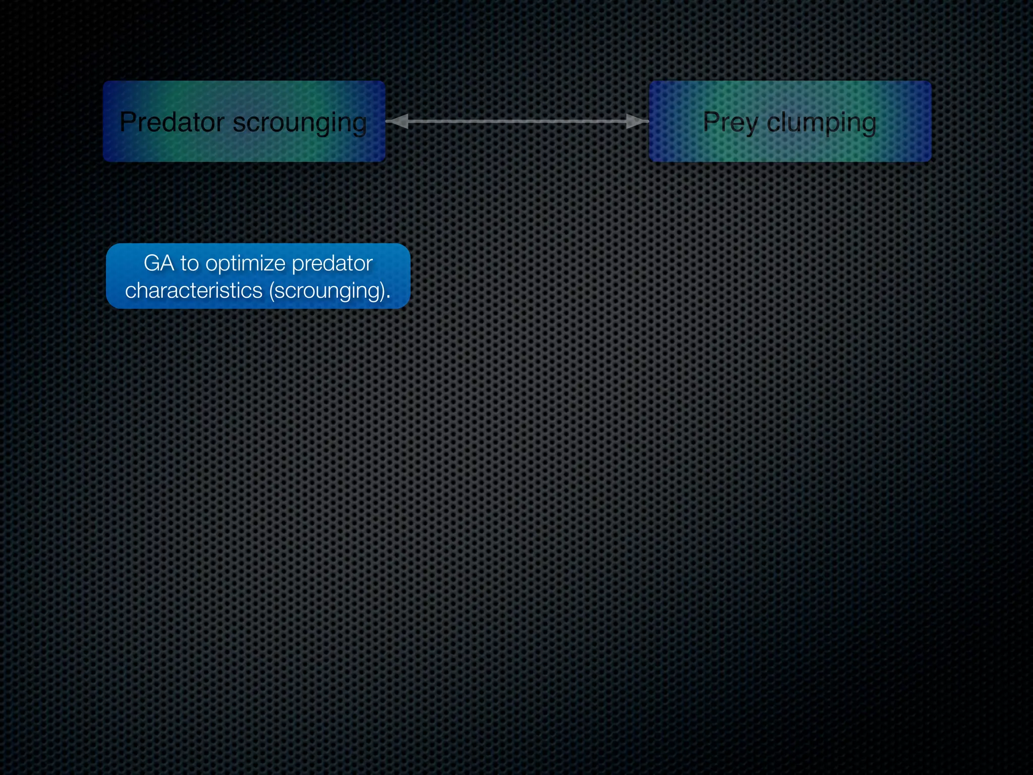
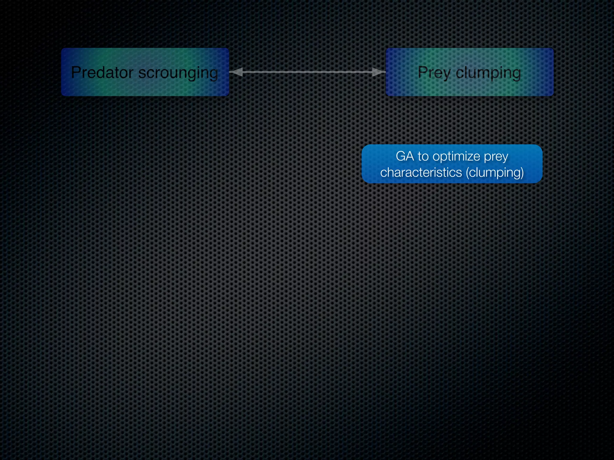
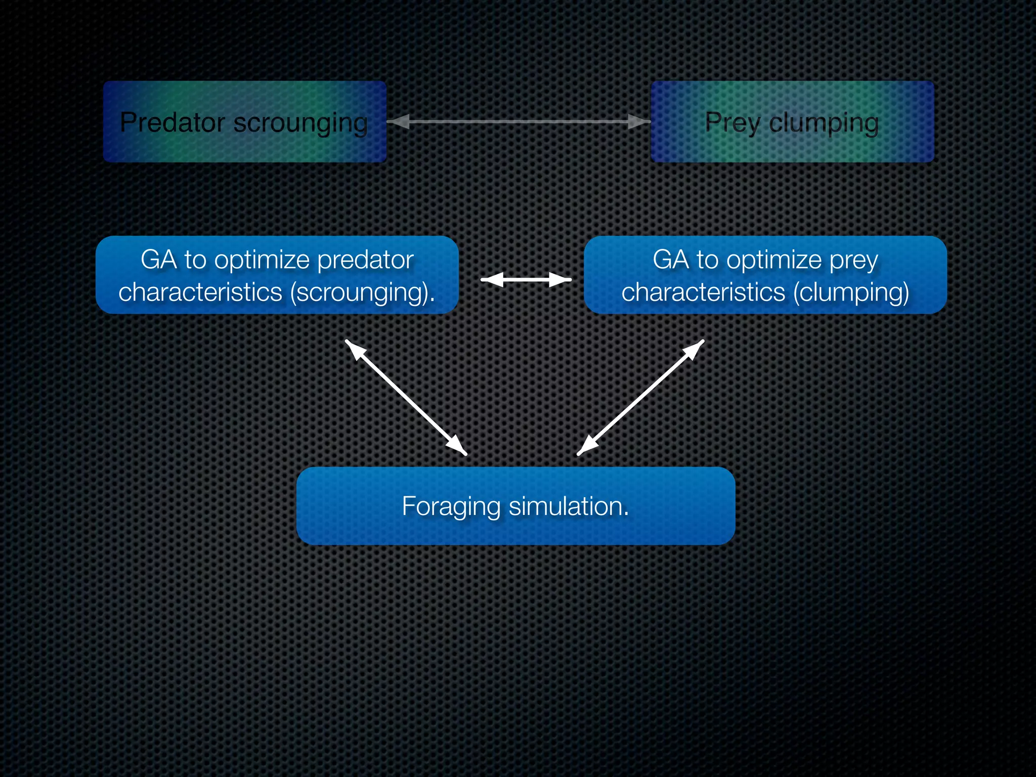
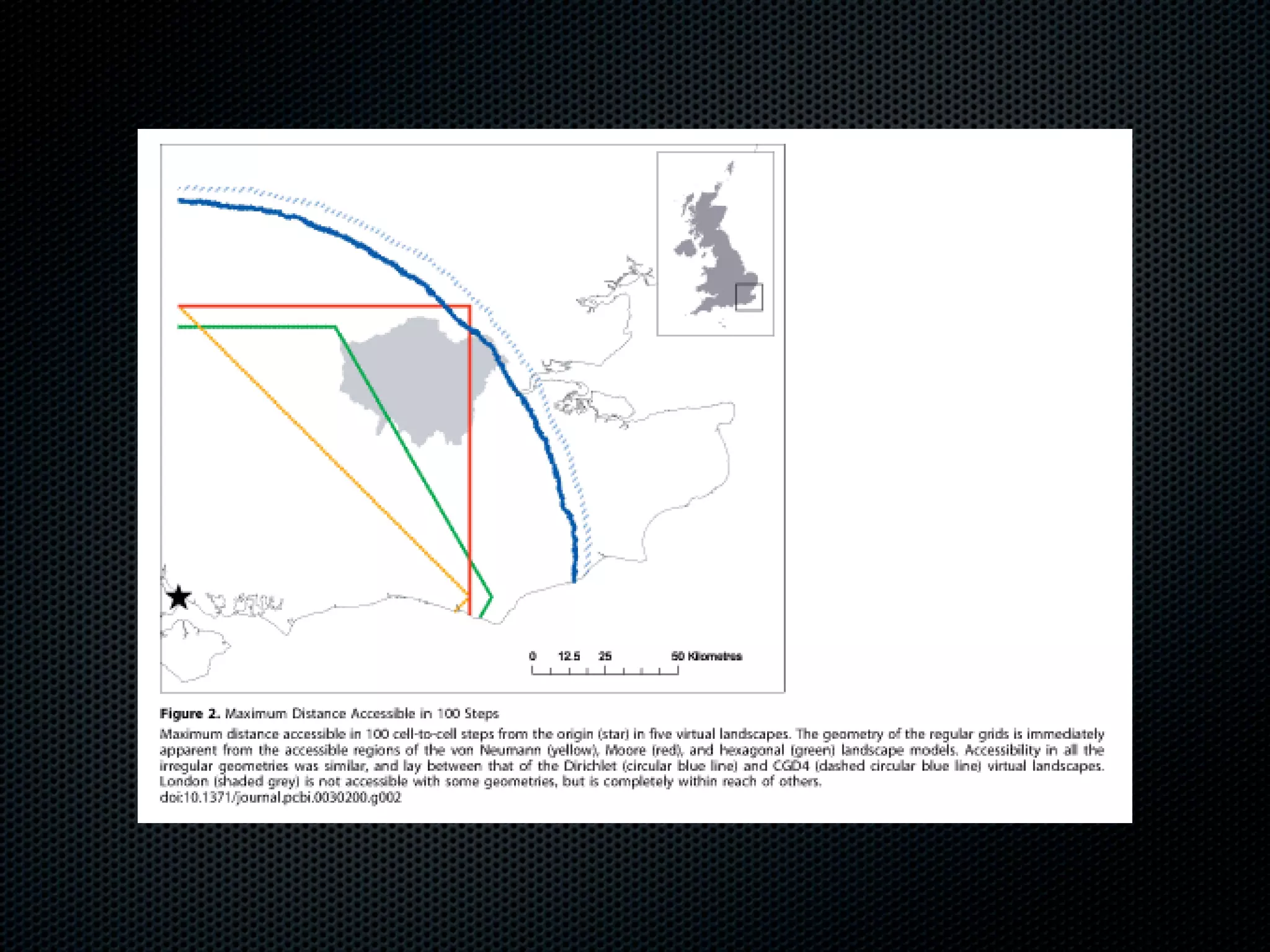
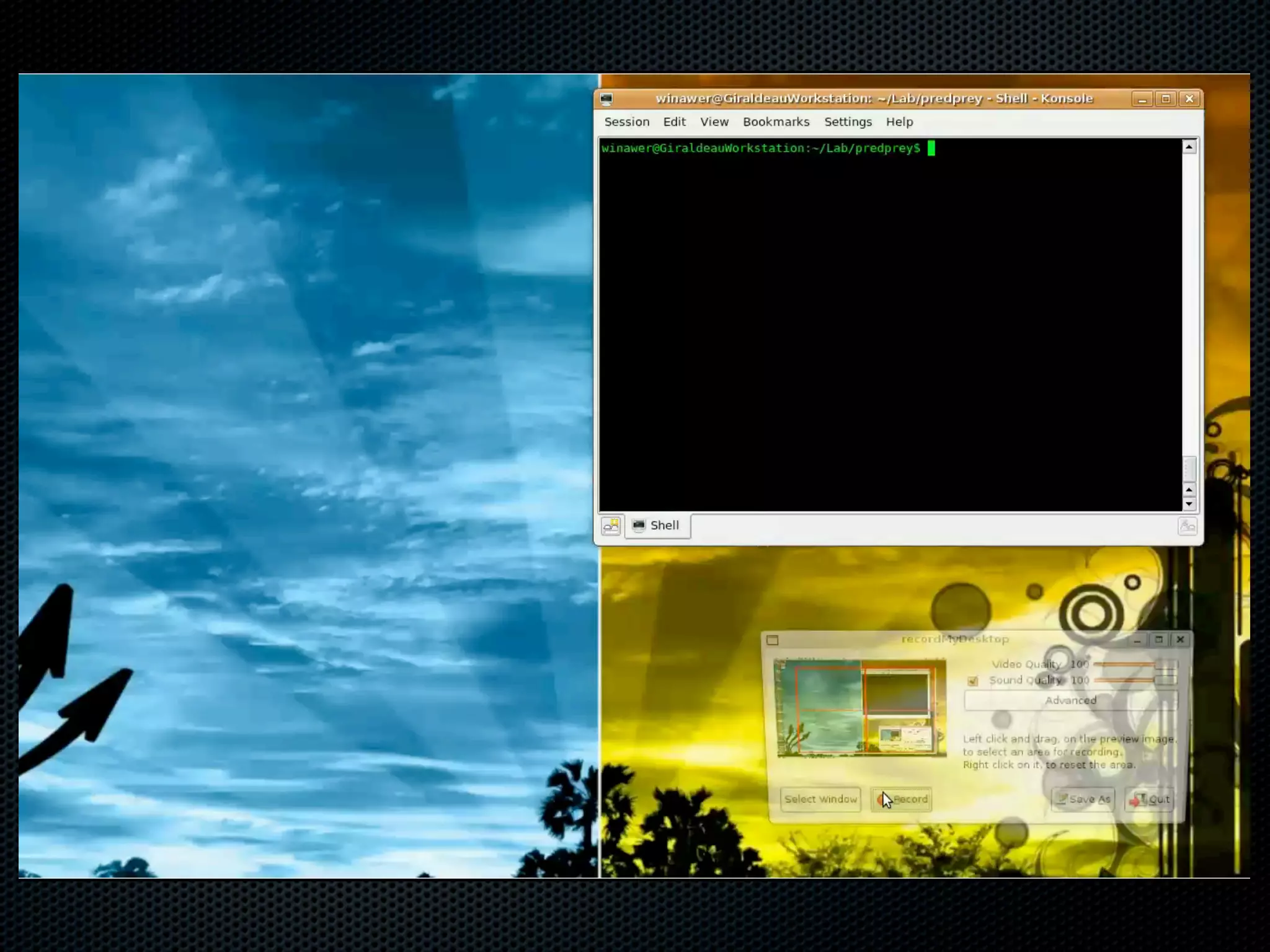
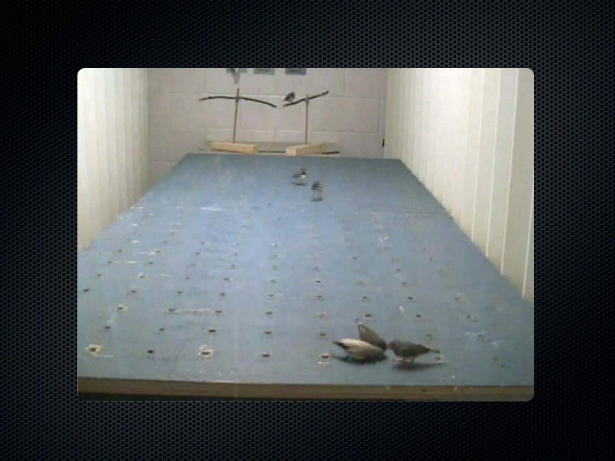
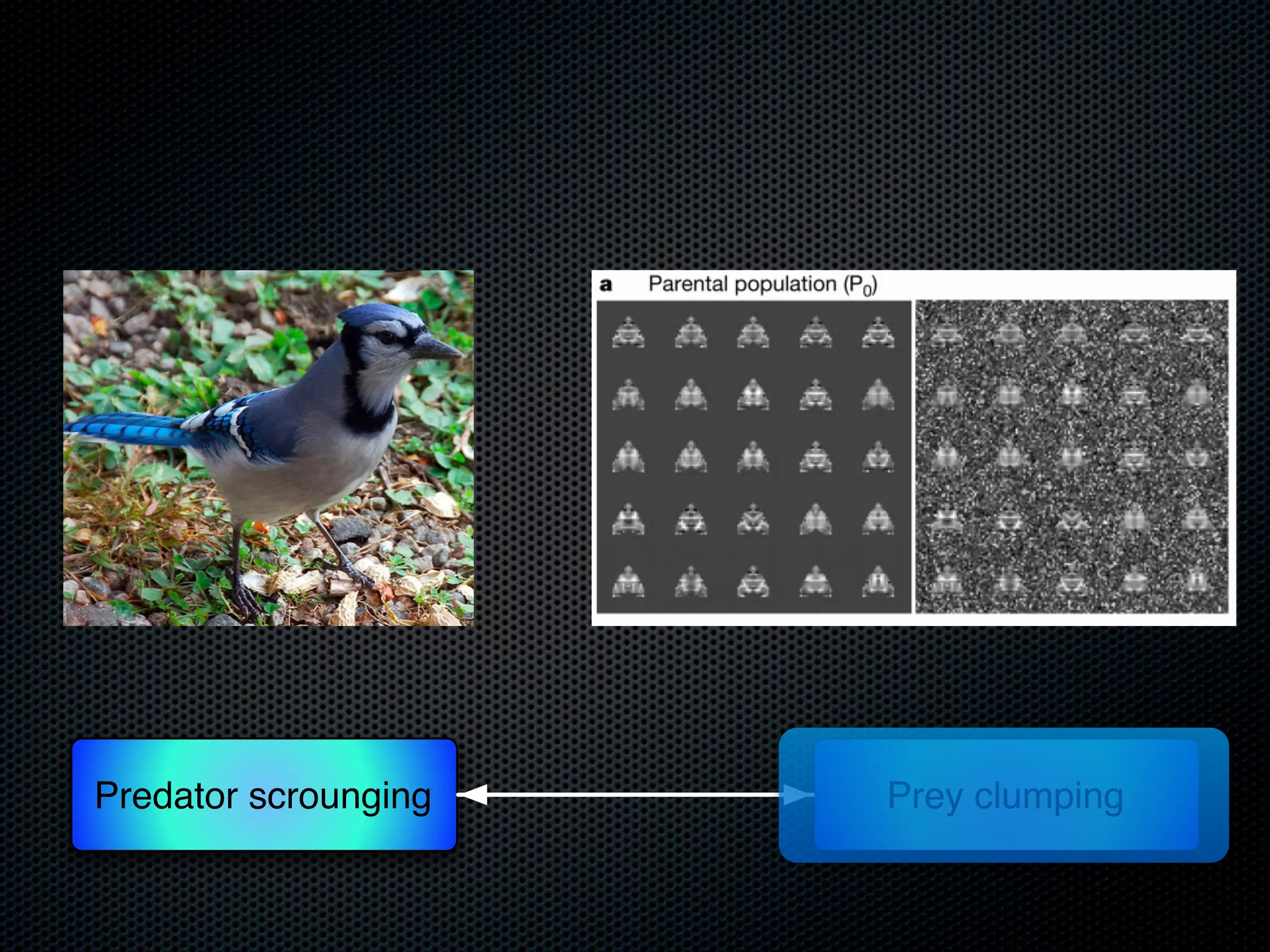
The document appears to be a Ph.D. proposal by Steven Hamblin that covers four chapters on foraging behavior and learning rules. Chapter 1 will discuss the evolution of learning rules for foraging. Chapter 2 will examine learning rules in more detail. Chapter 3 will consider the effects of landscape geometry on foraging. Chapter 4 will analyze predator-prey coevolution through changes in predator scrounging behavior and prey clumping habits. The proposal involves using genetic algorithms and foraging simulations to optimize learning rule parameters and population dynamics over time.

1. Ph.D proposal
steven hamblin

4. +
=
?

8. Social foraging
Equilibrium
behaviour
Learning

9. Producer

10. Scrounger
Producers

13. Chapter 1: Evolution of learning rules for foraging.

14. Chapter 1: Evolution of learning rules for foraging.
Chapter 2: Learning rules, the next step.

15. Chapter 1: Evolution of learning rules for foraging.
Chapter 2: Learning rules, the next step.
Chapter 3: Landscape geometry and foraging.

16. Chapter 1: Evolution of learning rules for foraging.
Chapter 2: Learning rules, the next step.
Chapter 3: Landscape geometry and foraging.
Chapter 4: Predator-prey coevolution.

17. Chapter 1:
Evolution of learning rules.

19. Scrounger
Producers

26. Rules

27. Rules
Relative payoff sum

28. Rules
Relative payoff sum
Perfect Memory

29. Rules
Relative payoff sum
Perfect Memory
Linear Operator

30. Relative
Payoff Sum?
Si (t) = xSi (t
1) + (1
Perfect
Memory?
Si (t) =
Linear
Operator?
Si (t) = xSi (t
x)ri + Pi (t)
+ Ri (t)/(⇥ + Ni (t))
1) + (1
x)Pi (t)

31. Relative
Payoff Sum?
Si (t) = xSi (t
1) + (1
Perfect
Memory?
Si (t) =
Linear
Operator?
Si (t) = xSi (t
x)ri + Pi (t)
+ Ri (t)/(⇥ + Ni (t))
1) + (1
x)Pi (t)

32. Relative
Payoff Sum?
Si (t) = xSi (t
1) + (1
Perfect
Memory?
Si (t) =
Linear
Operator?
Si (t) = xSi (t
x)ri + Pi (t)
+ Ri (t)/(⇥ + Ni (t))
1) + (1
x)Pi (t)
Multiple stable rules with multiple parameters?

33. Perfect
Memory?
Relative
Payoff Sum?
Linear
Operator?

34. Agent Start
Produce or
scrounge?
Produce
At a patch
with food?
Scrounge
No
Move
randomly
No
Any
conspecifics
feeding?
Yes
Feed
No
Move to
closest
Still food in
patch?
Yes
There yet?
Yes
No
Feed
Closest still
feeding?
Yes
No

35. Foraging grid is a
variable-sized square
grid with movement in
the 4 cardinal directions.
Agent Start
Produce or
scrounge?
Produce
At a patch
with food?
Scrounge
No
Move
randomly
No
Number of patches and
number of agents kept
to 20% and 10% of grid
size.
Any
conspecifics
feeding?
Yes
Feed
No
Move to
closest
Still food in
patch?
Yes
There yet?
Yes
No
Feed
Closest still
feeding?
Yes
No
Thus: 40x40 grid would
have 320 patches and
160 agents

36. Genetic Algorithms
Algorithms that
simulate evolution to
solve optimization
problems.

37. Initial population
Measure fitness
> n generations
Select for
reproduction
Mutation
Exit

38. Genetic algorithm to optimize parameters and
simulate population dynamics.
Foraging / Learning rule simulation.

39. Chapter 2:
Learning rules, the next step.

40. Si (t) = xSi (t
1) + (1
Perfect
Memory?
Si (t) = xSi (t
x)ri + Pi (t)
Si (t) =
1) + (1
Relative
Payoff Sum?
+ Ri (t)/(⇥ + Ni (t))
x)Pi (t)
Linear
Operator?

44. Initial population
Measure fitness
> n generations
Select for
reproduction
Mutation
Exit

47. Genetic algorithm to optimize parameters and
simulate population dynamics.
Foraging / Learning rule simulation.

48. Genetic programming to optimize rule structure.
Genetic algorithm to optimize parameters and
simulate population dynamics.
Foraging / Learning rule simulation.

49. Chapter 3:
Landscape geometry and foraging.

55. +

57. Foraging simulation.

58. Foraging simulation.
Swappable grids (Moore / VN / Hex / Dirichlet)

59. Genetic algorithm to optimize parameters and
simulate population dynamics.
Foraging simulation.
Swappable grids (Moore / VN / Hex / Dirichlet)

60. Chapter 4:
Predator-prey coevolution.

62. Predator scrounging
Prey clumping

63. Predator scrounging
Prey clumping

64. Predator scrounging
Prey clumping

66. Predator
characteristic
Prey
characteristic

68. Predator
characteristic
Prey
characteristic

69. Predator scrounging
Prey clumping

70. Predator scrounging
Prey clumping
Foraging simulation.

71. Predator scrounging
GA to optimize predator
characteristics (scrounging).
Prey clumping

72. Predator scrounging
Prey clumping
GA to optimize prey
characteristics (clumping)

73. Predator scrounging
Prey clumping
GA to optimize predator
characteristics (scrounging).
GA to optimize prey
characteristics (clumping)
Foraging simulation.

74. Finis. Questions?

80. Predator scrounging
Prey clumping

81. +
Before
ß
+
*
x
*
-
ß
1
∆
x
+
After
ß
+
+
x
*
-
ß
1
∆
x

82. Relative Payoff Sum
Si (t) = xSi (t
1) + (1
x)ri + Pi (t)
where 0 < x < 1 is a memory factor,
ri > 0 is the residual value associated with alternative i,
Pi (t) is the payo to alternative i at time t, and
Si (t) is the value that the animal places on the behavioural alternative i at
time t.

83. Relative Payoff Sum
Si (t) = xSi (t
1) + (1
x)ri + Pi (t)
where 0 < x < 1 is a memory factor,
ri > 0 is the residual value associated with alternative i,
Pi (t) is the payo to alternative i at time t, and
Si (t) is the value that the animal places on the behavioural alternative i at
time t.

84. Relative Payoff Sum
Si (t) = xSi (t
1) + (1
x)ri + Pi (t)
where 0 < x < 1 is a memory factor,
ri > 0 is the residual value associated with alternative i,
Pi (t) is the payo to alternative i at time t, and
Si (t) is the value that the animal places on the behavioural alternative i at
time t.

85. Relative Payoff Sum
Si (t) = xSi (t
1) + (1
x)ri + Pi (t)
where 0 < x < 1 is a memory factor,
ri > 0 is the residual value associated with alternative i,
Pi (t) is the payo to alternative i at time t, and
Si (t) is the value that the animal places on the behavioural alternative i at
time t.

86. Relative Payoff Sum
Si (t) = xSi (t
1) + (1
x)ri + Pi (t)
where 0 < x < 1 is a memory factor,
ri > 0 is the residual value associated with alternative i,
Pi (t) is the payo to alternative i at time t, and
Si (t) is the value that the animal places on the behavioural alternative i at
time t.

87. Perfect Memory
Si (t) =
+ Ri (t)/(⇥ + Ni (t))
where Ri (t) is the cumulative payo s from alternative i to time t,
Ni (t) is the number of time periods from the beginning in which the option
was selected,
and ⇥ are parameters.

88. Perfect Memory
Si (t) =
+ Ri (t)/(⇥ + Ni (t))
where Ri (t) is the cumulative payo s from alternative i to time t,
Ni (t) is the number of time periods from the beginning in which the option
was selected,
and ⇥ are parameters.

89. Perfect Memory
Si (t) =
+ Ri (t)/(⇥ + Ni (t))
where Ri (t) is the cumulative payo s from alternative i to time t,
Ni (t) is the number of time periods from the beginning in which the option
was selected,
and ⇥ are parameters.

90. Perfect Memory
Si (t) =
+ Ri (t)/(⇥ + Ni (t))
where Ri (t) is the cumulative payo s from alternative i to time t,
Ni (t) is the number of time periods from the beginning in which the option
was selected,
and ⇥ are parameters.

91. Linear Operator
Si (t) = xSi (t
1) + (1
x)Pi (t)
where 0 < x < 1 is a memory factor,
Pi (t) is the payo to alternative i at time t, and
Si (t) is the value that the animal places on the behavioural alternative i at
time t.