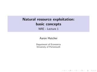
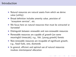
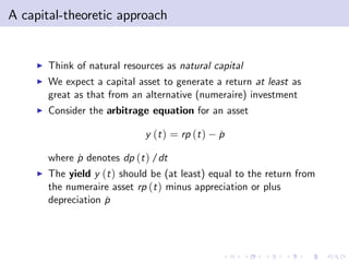


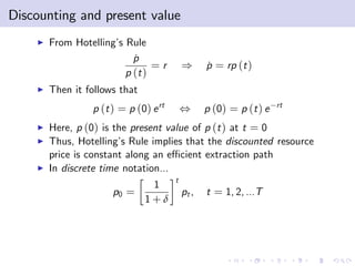
![A simple two-period resource allocation problem
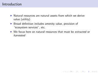
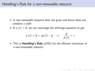
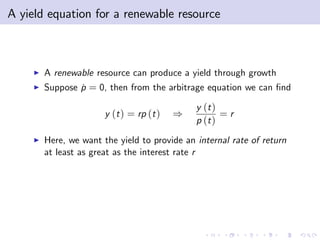
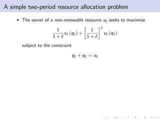
I The owner of a non-renewable resource x0 seeks to maximise
2
1 1
v1 (q1 ) + v2 (q2 )
1+δ 1+δ
subject to the constraint
q1 + q2 = x0
I The Lagrangian function for this problem is
2
1 1
L v1 (q1 ) + v2 (q2 ) + λ [x0 q1 q2 ]
1+δ 1+δ](https://image.slidesharecdn.com/nre-slides-1-100430053841-phpapp01/85/Natural-resource-exploitation-basic-concepts-37-320.jpg)
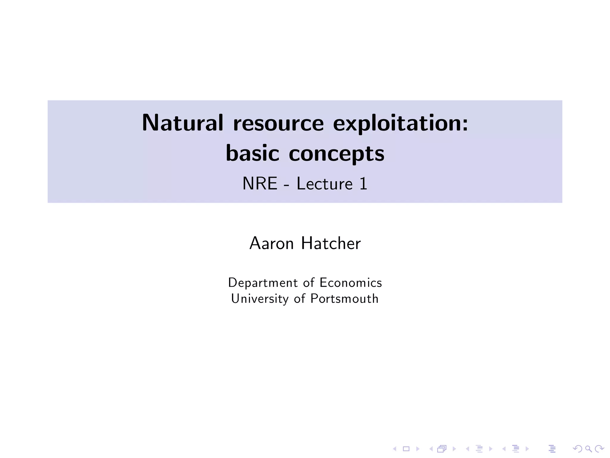
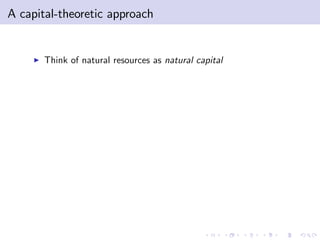
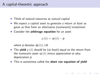
![A simple two-period resource allocation problem
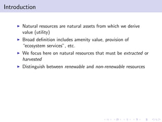
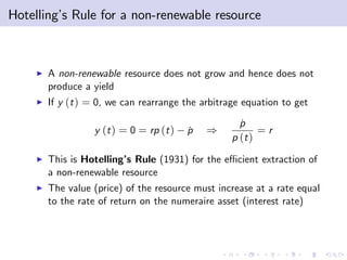
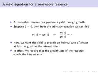
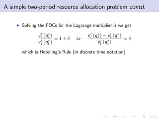
I The owner of a non-renewable resource x0 seeks to maximise
2
1 1
v1 (q1 ) + v2 (q2 )
1+δ 1+δ
subject to the constraint
q1 + q2 = x0
I The Lagrangian function for this problem is
2
1 1
L v1 (q1 ) + v2 (q2 ) + λ [x0 q1 q2 ]
1+δ 1+δ
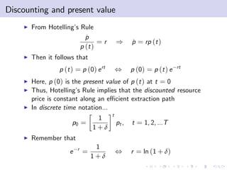
I The two …rst order (necessary) conditions are
2
1 1
v 0 (q ) λ = 0, 0
v2 (q2 ) λ=0
1+δ 1 1 1+δ](https://image.slidesharecdn.com/nre-slides-1-100430053841-phpapp01/85/Natural-resource-exploitation-basic-concepts-38-320.jpg)
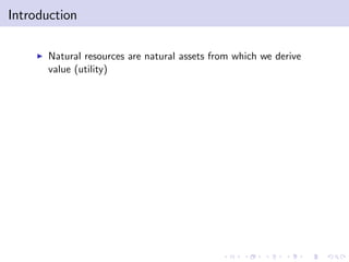
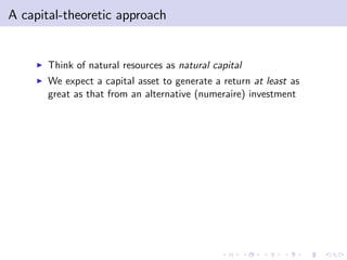
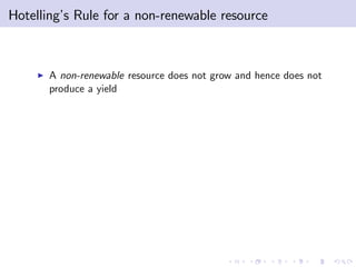
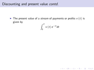
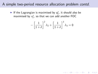
![A simple two-period resource allocation problem contd.
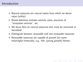
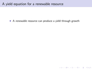
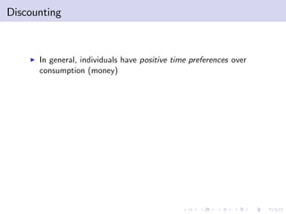
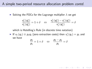
I Instead, we could attach a multiplier to a stock constraint at
each point in time
2
1 1 1
L v1 (q1 ) + v2 (q2 ) + λ1 [x0 x1 ]
1+δ 1+δ 1+δ
2 3
1 1
+ λ 2 [ x1 q1 x2 ] + λ3 [x2 q2 ]
1+δ 1+δ](https://image.slidesharecdn.com/nre-slides-1-100430053841-phpapp01/85/Natural-resource-exploitation-basic-concepts-42-320.jpg)
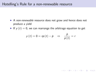
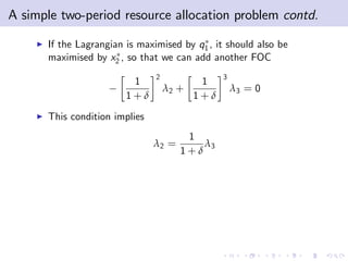
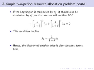
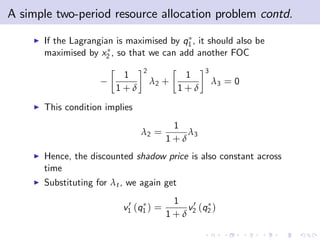
![A simple two-period resource allocation problem contd.
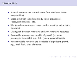
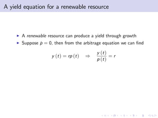
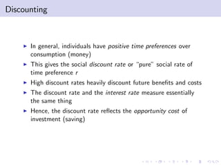
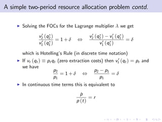
I Instead, we could attach a multiplier to a stock constraint at
each point in time
2
1 1 1
L v1 (q1 ) + v2 (q2 ) + λ1 [x0 x1 ]
1+δ 1+δ 1+δ
2 3
1 1
+ λ 2 [ x1 q1 x2 ] + λ3 [x2 q2 ]
1+δ 1+δ
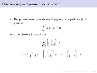
I The FOCs for q1 and q2 are now
2
1 1
v 0 (q ) λ2 = 0
1+δ 1 1 1+δ
2 3
1 0 1
v2 (q2 ) λ3 = 0
1+δ 1+δ](https://image.slidesharecdn.com/nre-slides-1-100430053841-phpapp01/85/Natural-resource-exploitation-basic-concepts-43-320.jpg)
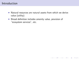
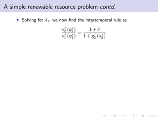
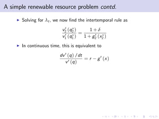
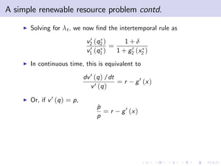
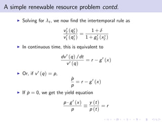
![A simple renewable resource problem
I We can set the problem in terms of a renewable resource by
incorporating a growth function gt (xt ) into each of the stock
constraints
t
1
λt [xt 1 + gt 1 (xt 1) qt 1 xt ]
1+δ](https://image.slidesharecdn.com/nre-slides-1-100430053841-phpapp01/85/Natural-resource-exploitation-basic-concepts-48-320.jpg)
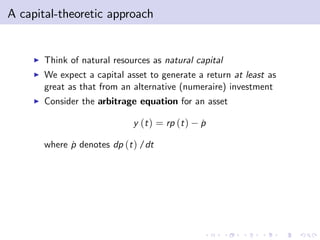
![A simple renewable resource problem
I We can set the problem in terms of a renewable resource by
incorporating a growth function gt (xt ) into each of the stock
constraints
t
1
λt [xt 1 + gt 1 (xt 1) qt 1 xt ]
1+δ
I Solving the Lagrangian as before, we get
2 2 3
1 0 1 1 0 1
v1 (q1 ) = λ2 , v2 (q2 ) = λ3
1+δ 1+δ 1+δ 1+δ
and
2 3
1 1 0
λ2 = λ3 1 + g2 (x2 )
1+δ 1+δ](https://image.slidesharecdn.com/nre-slides-1-100430053841-phpapp01/85/Natural-resource-exploitation-basic-concepts-49-320.jpg)

The document discusses the fundamental concepts of natural resource exploitation, focusing on the difference between renewable and non-renewable resources, and their economic implications. It includes the capital-theoretic approach to natural resources, emphasizing the importance of efficient intertemporal allocation, investment returns, and discount rates. The document also elaborates on Hotelling’s rule, which addresses the optimal extraction rate for non-renewable resources.


