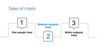
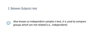
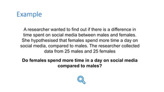
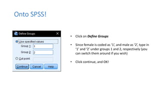
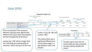
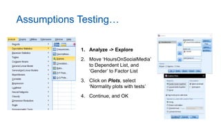
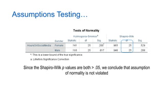
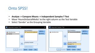
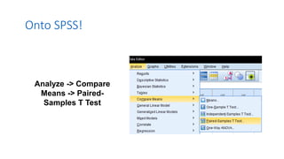
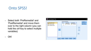
1. The document discusses different types of t-tests including the between subjects t-test. 2. It provides an example of using a between subjects t-test to compare time spent on social media between males and females, with results showing females spent significantly more time than males. 3. Guidance is given on testing assumptions, conducting the t-test in SPSS, and interpreting the results including a significant difference found between the groups.

1. REVISION DMME 5083
STATISTICS FOR EDUCATIONAL RESEARCH

2. Types of t-tests
One sample t-test
Between subjects
t-test
Within subjects
t-test
1
2
3

3. 2. Between Subjects t-test
Also known as independent samples t-test, it is used to compare
groups which are not related (i.e., independent)

4. A researcher wanted to find out if there is a difference in
time spent on social media between males and females.
She hypothesised that females spend more time a day on
social media, compared to males. The researcher collected
data from 25 males and 25 females
Do females spend more time in a day on social media
compared to males?
Example

5. Assumptions Testing…
Before conducting the t-test, we need to first test the
assumption of normality

6. Assumptions Testing…
1. Analyze -> Explore
2. Move ‘HoursOnSocialMedia’
to Dependent List, and
‘Gender’ to Factor List
3. Click on Plots, select
‘Normality plots with tests’
4. Continue, and OK

7. Assumptions Testing…
Since the Shapiro-Wilk p values are both > .05, we conclude that assumption
of normality is not violated

8. Onto SPSS!
• Analyze -> Compare Means -> Independent Samples T Test
• Move ‘HoursOnSocialMedia’ to the right column as the Test Variable
• Select ‘Gender’ as the Grouping Variable

9. Onto SPSS!
• Click on Define Groups
• Since female is coded as ‘1’, and male as ‘2’, type in
‘1’ and ‘2’ under groups 1 and 2, respectively (you
can switch them around if you wish)
• Click continue, and OK!

10. This is to evaluate if the variances
between 2 groups were significantly
different from each other (Assumption
test for homogeneity of Variance)
p-value was .378, which is larger than
.05, indicating assumed equality of
variances. Hence we focus on this row
Onto SPSS!
t value = 8.12, df = 48, and
p value <.001.
This means there was a
significant difference on
social media usage in a
day between males and
females
Females spent more time on
social media per day compared
to males (almost double the
time!)

11. Onto SPSS!
Analyze -> Compare
Means -> Paired-
Samples T Test

12. • Select both ‘PreRemedial’ and
‘PostRemedial’ and move them
over to the right column (you can
hold the ctrl key to select multiple
variables)
• OK!
Onto SPSS!

13. We can say that, on average, students who underwent remedial classes
improved their grades from 43.65 to 57.60 (check p value for statistical
significance)
Looking at the output file, we get a t
score = -5.834.
Onto SPSS!
This is the degrees of freedom (n -
number of pairs = 19)
p-value < .001 (smaller than the critical alpha .05).
We reject the null hypothesis. Therefore, we
conclude that scores before and after remedial
lessons were significantly different.

14. When can we use ANOVA?
• The t-test is used to compare the means of two-
groups.
• One-way ANOVA is used to compare the means of
two or more groups.
• We can use one-way ANOVA whenever the
dependent variable (DV) is numerical and the
independent variable (IV) is categorical.
• The independent variable in ANOVA is also called a
factor. 14

15. Examples
The following are situations where we can use
ANOVA:
• Testing the differences in blood pressure among
different groups of people (DV is blood pressure
and the group is the IV).
• Testing which type of social media affects hours of
sleep (type of social media used is the IV and hours
of sleep is the DV).
15

16. Assumptions of ANOVA
• The observations in each group are normally
distributed.
This can be tested by plotting the numerical variable
separately for each group and checking that they all have a
bell shape.
Alternatively, you could use the Shapiro-Wilk test for
normality.
16

17. Assumptions
• The groups have equal variances (i.e., homogeneity of
variance).
You can plot each group separately and check that they exhibit similar
variability.
Alternatively, you can use Levene’s test for homogeneity.
• The observations in each group are independent.
This could be assessed by common sense looking at the study design.
For example, if there is a participant in more than one group, your
observations are not independent.
17

18. Hypothesis Testing
ANOVA tests the null hypothesis:
H0 : The groups have equal means
versus the alternative hypothesis:
H1 : At least one group mean is different from the
other group means.
18
F-Test

19. ANOVA in SPSS
Example:
Is there a difference in optimism scores for young, middle-
aged and old participants?
Categorical IV - Age with 3 levels:
• 29 and younger
• Between 30 and 44
• 45 or above
Continuous DV – Optimism scores
19

20. ANOVA in SPSS
1. Click on Analyze, Compare Means, then One-
way ANOVA.
2. Click on your continuous dependent variable
(e.g., Total Optimism: toptim). Move this into the
box marked Dependent List by clicking on the
arrow button.
3. Click on your independent, categorical variable
(e.g., age 3 groups: agegp3). Move this into the
box labelled Factor.
20

21. ANOVA in SPSS
4. Click the Options button and click on
Descriptive, Homogeneity of variance test,
Brown-Forsythe, Welch test and Means plot.
5. For Missing Values, make sure there is a dot in
the option marked Exclude cases analysis by
analysis. Click on Continue.
6. Click on the button marked Post Hoc. Click on
Tukey.
7. Click on Continue and then OK.
21

22. ANOVA in SPSS
Interpreting the output:
1. Check that the groups have equal variances using Levene’s test for
homogeneity.
• Check the significance value (Sig.) for Levene’s test Based on Mean.
• If this number is greater than .05 you have not violated the assumption of
homogeneity of variance.
22

23. ANOVA in SPSS
Interpreting the output:
2. Check the significance of the ANOVA.
• If the Sig. value is less than or equal to .05, there is a significant difference
somewhere among the mean scores on your dependent variable for the
three groups.
• However, this does not tell us which group is different from which other
group.
23

24. ANOVA in SPSS
Interpreting the output:
3. ONLY if the ANOVA is significant, check the significance of the
differences between each pair of groups in the table labelled
Multiple Comparisons.
24

25. ANOVA in SPSS
Calculating effect size:
• In an ANOVA, effect size will tell us how large the difference between
groups is.
• We will calculate eta squared, which is one of the most common
effect size statistics.
25
Eta squared
=
Sum of squares between groups
Total sum of squares

26. ANOVA in SPSS
Calculating effect size:
26
179.07
8513.02
= .02
According to Cohen (1988):
Small effect: .01
Medium effect: .06
Large effect: .14

27. ANOVA in SPSS
Example results write-up:
A one way between-groups analysis of variance was conducted to explore the impact of
age on levels of optimism. Participants were divided into three groups according to
their age (Group 1: 29yrs or less; Group 2: 30 to 44yrs; Group 3: 45yrs and above).
There was a statistically significant difference at the p < .05 level in optimism scores for
the three age groups: F (2, 432) = 4.6, p = .01. Despite reaching statistical significance,
the actual difference in mean scores between the groups was quite small. The effect
size, calculated using eta squared, was .02. Post-hoc comparisons using the Tukey HSD
test indicated that the mean score for Group 1 (M = 21.36, SD = 4.55) was significantly
different from Group 3 (M = 22.96, SD = 4.49).
27

28. ANOVA in SPSS
28
Note: Results are usually rounded to two decimal
places

29. Bivariate Statistical Matrix

30. Correlation
Is there a statistically significant association between numerical (continuous) variables?
Ex: HH expenditure share on food & HHsize
Analyze => Correlate => Bivariate

31. Correlation
Is there a statistically significant association between numerical (continuous) variables?
Ex: HH expenditure share on food & HHsize
Analyze => Correlate => Bivariate

32. Correlation
1- Correlations Coefficient - r
• In a range from -1 to +1 (Direction) moving in the same
direction or opposite direction.
• r= 0.2 (weak + association or correlation)
• r= - 0.8 (strong - association or correlation)
2- P < 0.05 (significance cutoff point)
What to look at ?
3- Interpretation
The variables are significantly associated (or behaving together ) either at the
same direction or in opposite direction. NO CAUSALITY.. ! No one makes the
other to happen..!

33. Correlation SPSS Output
Is there a statistically significant association between numerical (continuous) variables?
Ex: Age and income
Analyze => Correlate => Bivariate
Correlations Coefficient -
r
P <
0.05

34. Regression
• Regression analysis is the statistical test used to assess the CAUSALITY .. How variable affect the other.
• Regression analysis is the test to be used to say that the variable X induce the variable Y to happen with the magnitude of
Z.
• We are using a simple linear regression to assess the impact of one independent variable on another dependent variable.
How the HH size impact the FCS or the expenditure on food…?

35. Outcome
Variable
Are the observations independent or correlated?
Alternatives if the normality
assumption is violated (and
small sample size):
independent correlated
Continuous
(e.g. pain
scale,
cognitive
function)
Ttest: compares means between
two independent groups
ANOVA: compares means
between more than two
independent groups
Pearson’s correlation
coefficient (linear
correlation): shows linear
correlation between two continuous
variables
Linear regression:
multivariate regression technique
used when the outcome is
continuous; gives slopes
Paired ttest: compares means
between two related groups (e.g.,
the same subjects before and after)
Repeated-measures
ANOVA: compares changes over
time in the means of two or more
groups (repeated measurements)
Mixed models/GEE
modeling: multivariate regression
techniques to compare changes over
time between two or more groups;
gives rate of change over time
Non-parametric statistics
Wilcoxon sign-rank test:
non-parametric alternative to the
paired ttest
Wilcoxon sum-rank test
(=Mann-Whitney U test): non-
parametric alternative to the ttest
Kruskal-Wallis test: non-
parametric alternative to ANOVA
Spearman rank correlation
coefficient: non-parametric
alternative to Pearson’s correlation
coefficient

36. Scatter Plots of Data with Various
Correlation Coefficients
Y
X
Y
X
Y
X
Y
X
Y
X
r = -1 r = -.6 r = 0
r = +.3
r = +1
Y
X
r = 0
Slide from: Statistics for Managers Using Microsoft® Excel 4th Edition, 2004 Prentice-Hall

37. Y
X
Y
X
Y
Y
X
X
Linear relationships Curvilinear
relationships
Linear Correlation
Slide from: Statistics for Managers Using Microsoft® Excel 4th Edition, 2004 Prentice-Hall

38. Y
X
Y
X
Y
Y
X
X
Strong
relationships
Weak relationships
Linear Correlation
Slide from: Statistics for Managers Using Microsoft® Excel 4th Edition, 2004 Prentice-Hall

39. Linear Correlation
Y
X
Y
X
No relationship
Slide from: Statistics for Managers Using Microsoft® Excel 4th Edition, 2004 Prentice-Hall

40. Continuous outcome (means)
Outcome
Variable
Are the observations independent or correlated?
Alternatives if the normality
assumption is violated (and
small sample size):
independent correlated
Continuous
(e.g. pain
scale,
cognitive
function)
Ttest: compares means between
two independent groups
ANOVA: compares means
between more than two
independent groups
Pearson’s correlation
coefficient (linear
correlation): shows linear
correlation between two continuous
variables
Linear regression:
multivariate regression technique
used when the outcome is
continuous; gives slopes
Paired ttest: compares means
between two related groups (e.g.,
the same subjects before and after)
Repeated-measures
ANOVA: compares changes over
time in the means of two or more
groups (repeated measurements)
Mixed models/GEE
modeling: multivariate
regression techniques to compare
changes over time between two or
more groups; gives rate of change
over time
Non-parametric statistics
Wilcoxon sign-rank test:
non-parametric alternative to the
paired ttest
Wilcoxon sum-rank test
(=Mann-Whitney U test): non-
parametric alternative to the ttest
Kruskal-Wallis test: non-
parametric alternative to ANOVA
Spearman rank correlation
coefficient: non-parametric
alternative to Pearson’s correlation
coefficient

41. Linear regression
In correlation, the two variables are treated as
equals. In regression, one variable is considered
independent (=predictor) variable (X) and the other
the dependent (=outcome) variable Y.

42. Prediction
If you know something about X, this knowledge helps you
predict something about Y. (Sound familiar?…sound
like conditional probabilities?)

43. Multiple linear regression…
• What if age is a confounder here?
• Older men have lower vitamin D
• Older men have poorer cognition
• “Adjust” for age by putting age in the model:
• DSST score = intercept + slope1xvitamin D + slope2 xage

44. Multiple Linear Regression
• More than one predictor…
E(y)=  + 1*X + 2 *W + 3 *Z…
Each regression coefficient is the amount of change in the outcome
variable that would be expected per one-unit change of the
predictor, if all other variables in the model were held constant.

45. • A salesperson for a large car brand wants to determine whether
there is a relationship between an individual's income and the
price they pay for a car. As such, the individual's "income" is the
independent variable and the "price" they pay for a car is the
dependent variable. The salesperson wants to use this
information to determine which cars to offer potential customers
in new areas where average income is known.

46. This table provides the R and R2 values. The R value represents the simple
correlation and is 0.873 (the "R" Column), which indicates a high degree of
correlation. The R2 value (the "R Square" column) indicates how much of
the total variation in the dependent variable, Price, can be explained by the
independent variable, Income. In this case, 76.2% can be explained, which
is very large.

47. The next table is the ANOVA table, which reports how well the regression
equation fits the data (i.e., predicts the dependent variable) and is shown below:
This table indicates that the regression model predicts the dependent variable
significantly well. How do we know this? Look at the "Regression" row and go to
the "Sig." column. This indicates the statistical significance of the regression model
that was run. Here, p < 0.0005, which is less than 0.05, and indicates that, overall,
the regression model statistically significantly predicts the outcome variable (i.e., it
is a good fit for the data).

48. The Coefficients table provides us with the necessary information to
predict price from income, as well as determine whether income
contributes statistically significantly to the model (by looking at the "Sig."
column). Furthermore, we can use the values in the "B" column under the
"Unstandardized Coefficients" column

49. Dr. Said T. EL Hajjar
49
SPSS is a tool
-If you provide it with flower, it gives you honey
-If you provide it with rubbish, it gives you garbage
Thank you