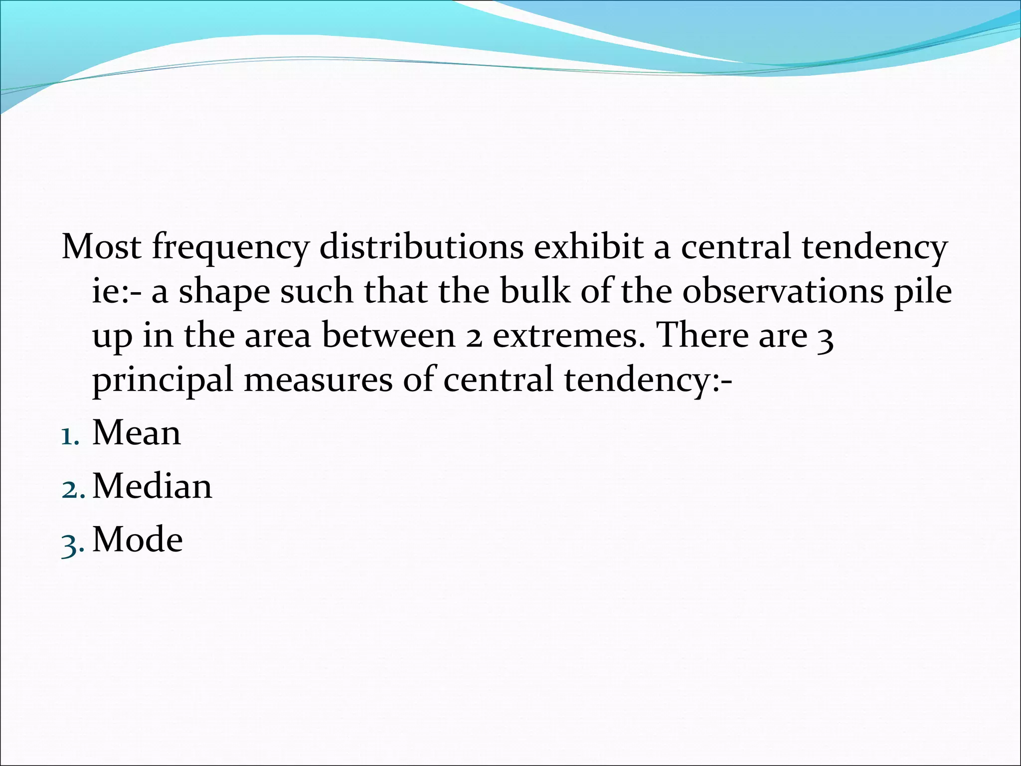
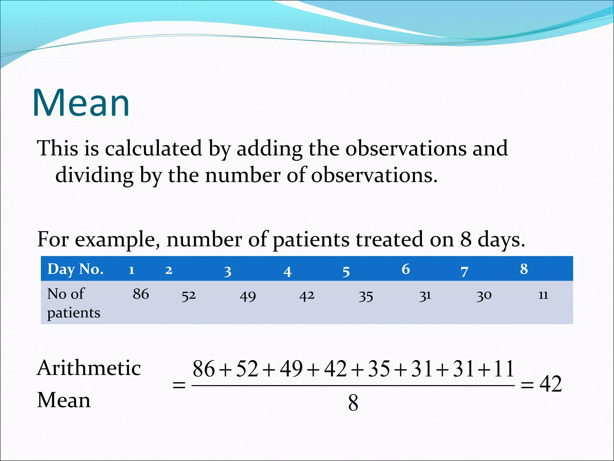
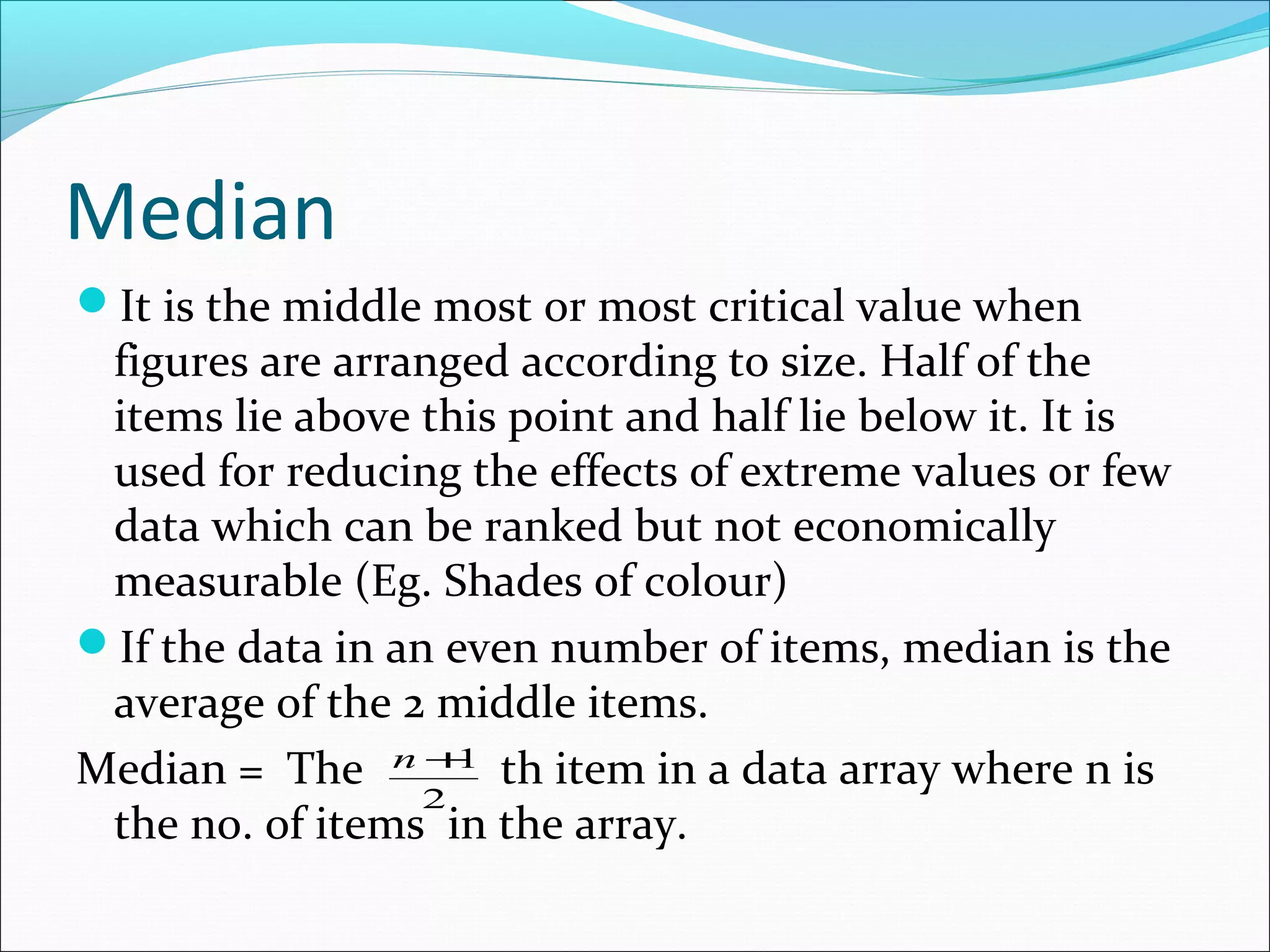
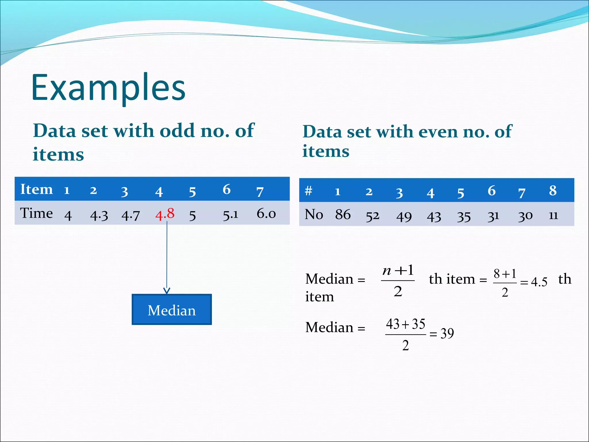
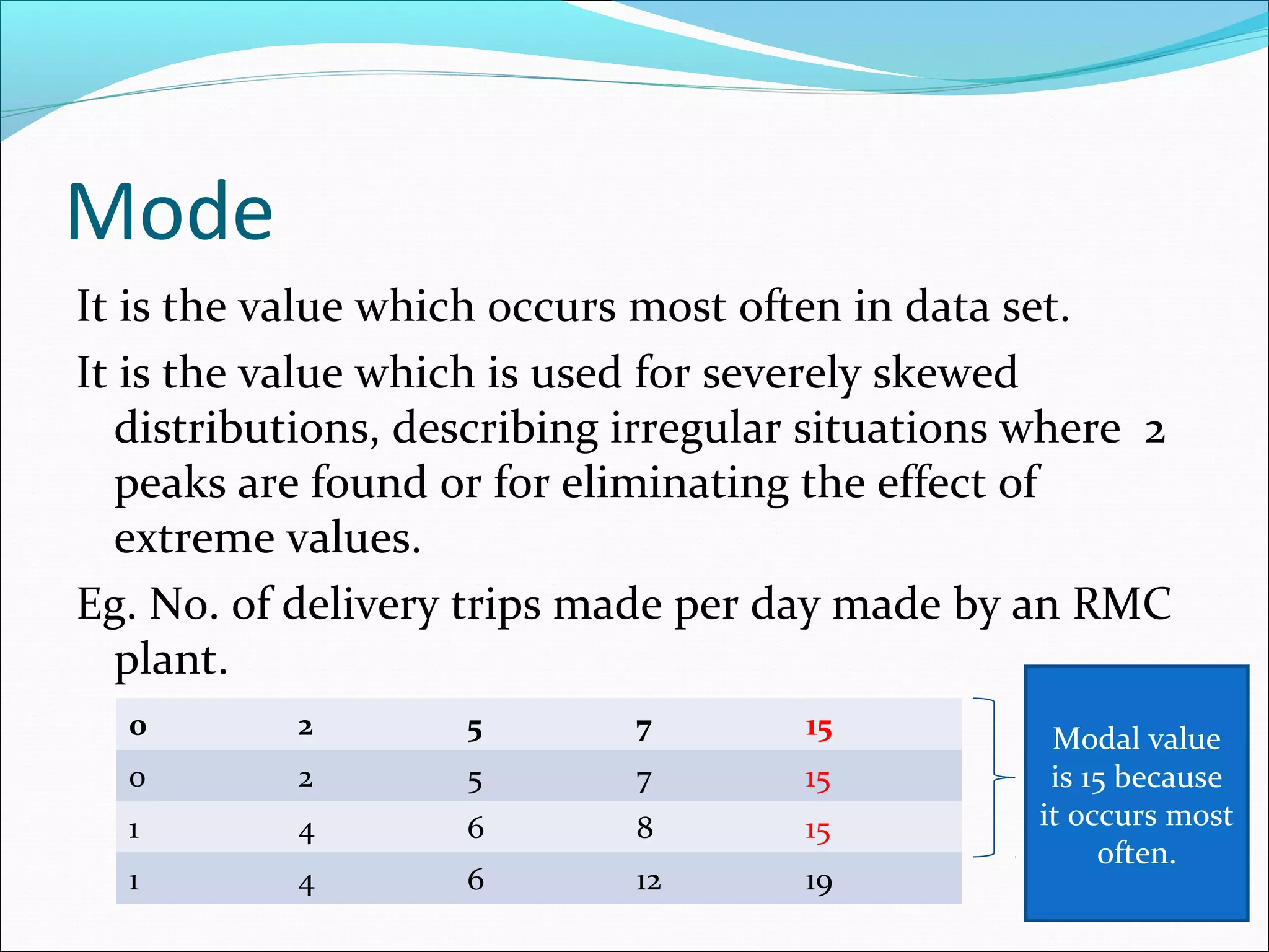
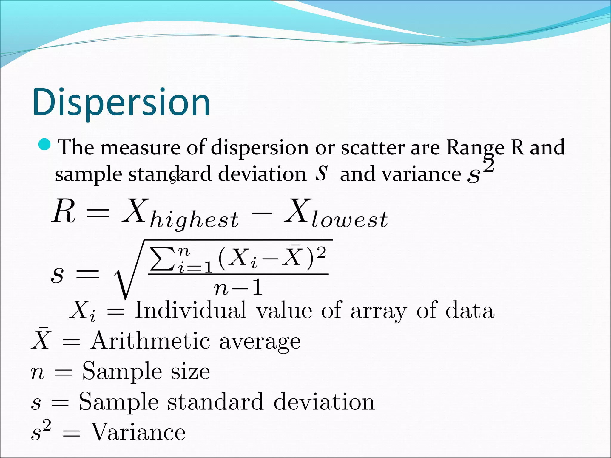
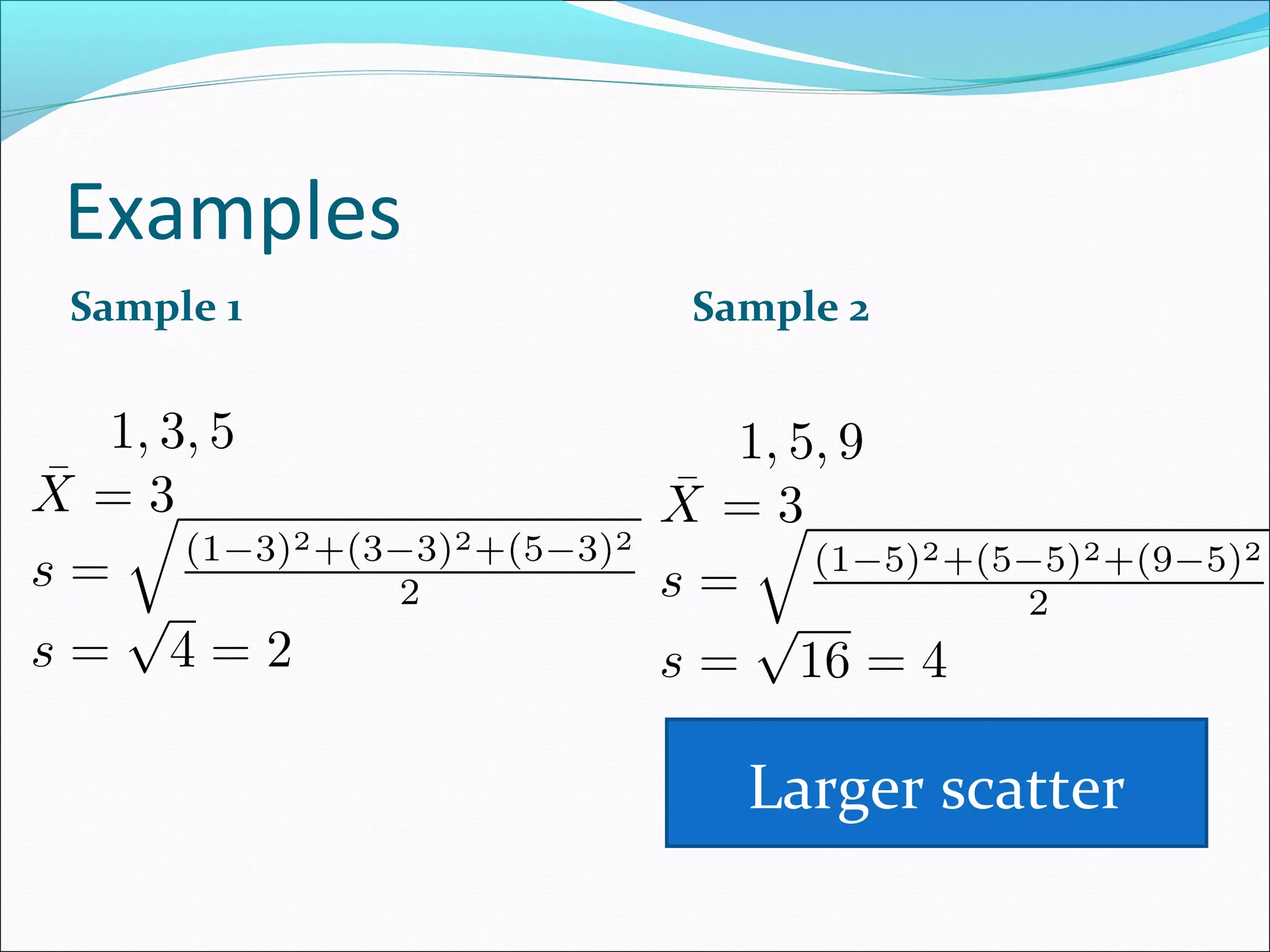
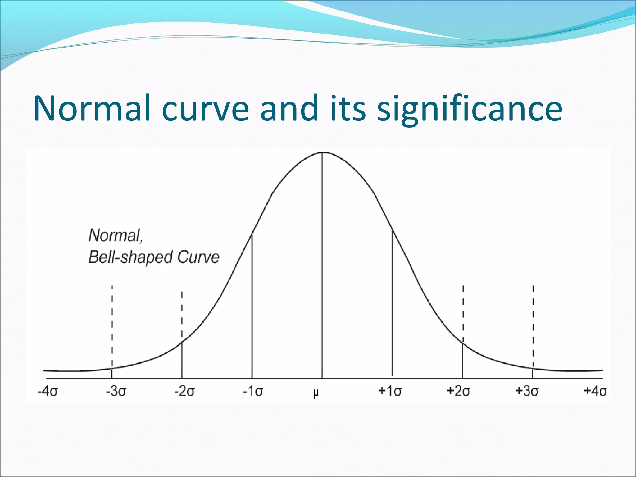
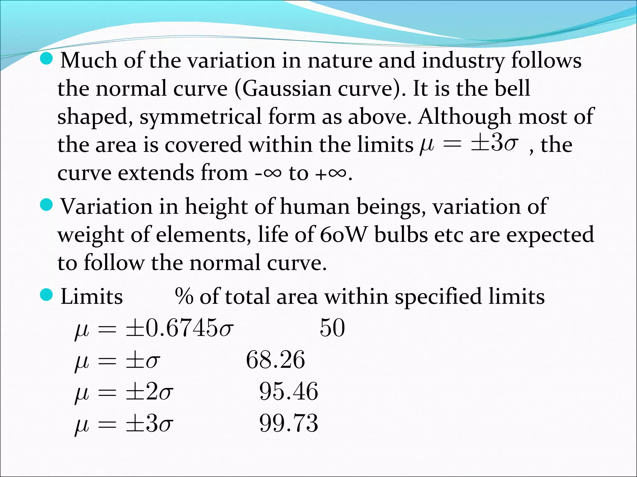
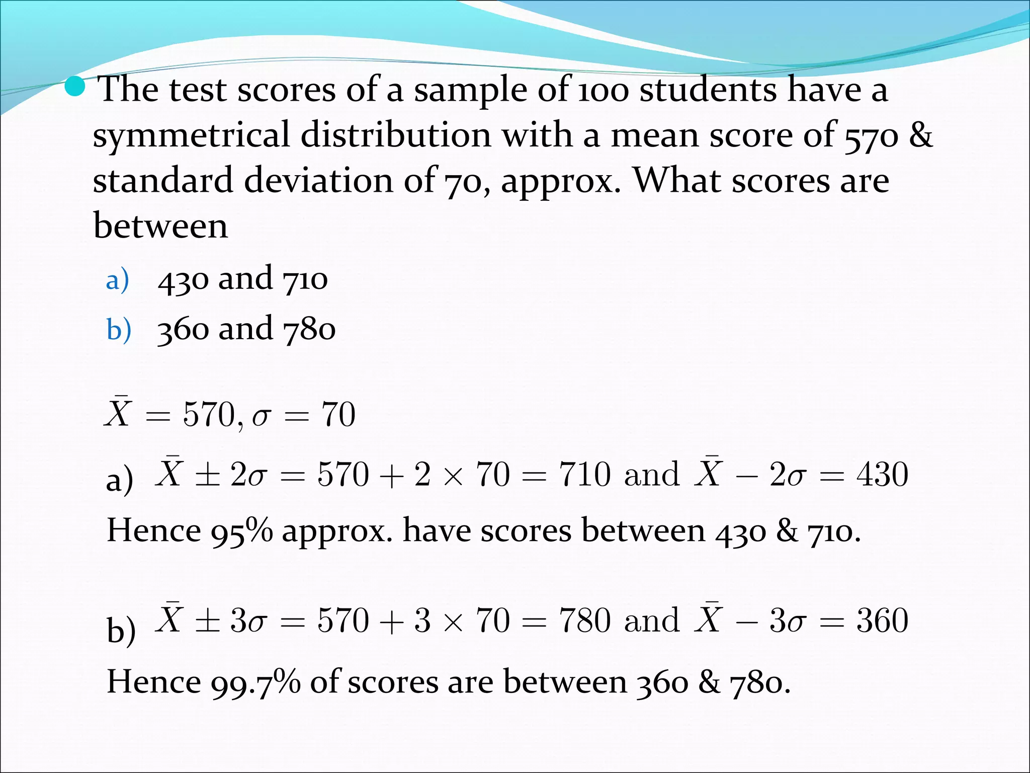
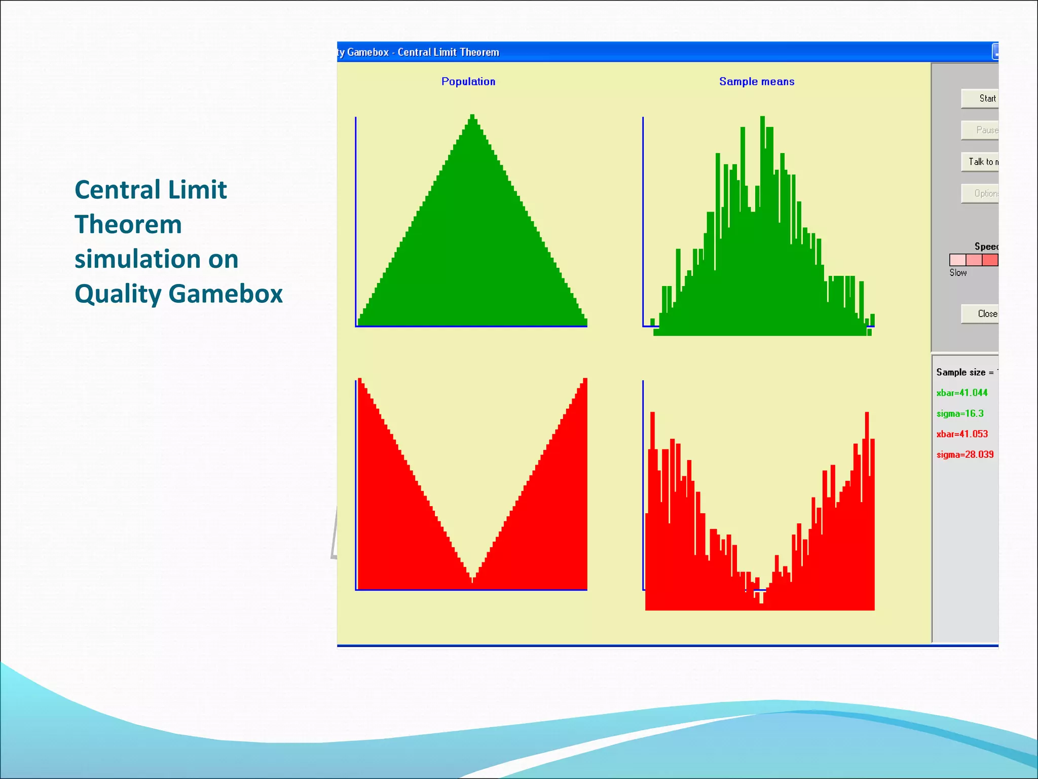
This document summarizes three measures of central tendency (mean, median, mode) and dispersion (range, standard deviation). It provides examples and explanations of how to calculate each measure. It also discusses the normal distribution curve and how it is used to describe variation in natural and industrial processes. The central limit theorem is introduced, stating that as sample size increases, the distribution of sample means approaches a normal distribution, regardless of the population distribution.

2. Most frequency distributions exhibit a central tendency
ie:- a shape such that the bulk of the observations pile
up in the area between 2 extremes. There are 3
principal measures of central tendency:1. Mean
2. Median
3. Mode

3. Mean
This is calculated by adding the observations and
dividing by the number of observations.
For example, number of patients treated on 8 days.
Day No.
1
No of
patients
86
Arithmetic
Mean
2
3
52
4
49
5
42
6
35
7
31
8
30
11
86 + 52 + 49 + 42 + 35 + 31 + 31 + 11
=
= 42
8

4. Median
It is the middle most or most critical value when
figures are arranged according to size. Half of the
items lie above this point and half lie below it. It is
used for reducing the effects of extreme values or few
data which can be ranked but not economically
measurable (Eg. Shades of colour)
If the data in an even number of items, median is the
average of the 2 middle items.
1
Median = The n + th item in a data array where n is
2
the no. of items in the array.

5. Examples
Data set with odd no. of
items
Item 1
2
3
Time 4
4.3 4.7
4
5
4.8 5
Median
Data set with even no. of
items
6
7
#
5.1
6.0
No 86 52
1
Median =
item
Median =
2
3
4
49 43
5
6
7
8
35
31
30
11
n +1
th item = 8 + 1 = 4.5 th
2
2
43 + 35
= 39
2

6. Mode
It is the value which occurs most often in data set.
It is the value which is used for severely skewed
distributions, describing irregular situations where 2
peaks are found or for eliminating the effect of
extreme values.
Eg. No. of delivery trips made per day made by an RMC
plant.
0
2
5
7
15
0
2
5
7
15
1
4
6
8
15
1
4
6
12
19
Modal value
is 15 because
it occurs most
often.

7. The modal value 15 inplies that the plant activity is
higher than 6.7 (which is mean). The mode tells us
that 15 is the most frequent no. of trip, but it fails to
let us know that most of the values are under 10.
A distribution in which the values of mean, median
and mode coincide is known as symmetrical
distribution. When they do not coincide, the
distribution is known as skewed or asymmetrical.
If distribution is moderately skewed,
Mean – Mode = 3(Mean-Median)

8. Dispersion
The measure of dispersion or scatter are Range R and
sample standard deviation
s
and variance

9. Examples
Sample 1
Sample 2
Larger scatter

10. Normal curve and its significance

11. Much of the variation in nature and industry follows
the normal curve (Gaussian curve). It is the bell
shaped, symmetrical form as above. Although most of
the area is covered within the limits
, the
curve extends from -∞ to +∞.
Variation in height of human beings, variation of
weight of elements, life of 60W bulbs etc are expected
to follow the normal curve.
Limits
% of total area within specified limits

12. The test scores of a sample of 100 students have a
symmetrical distribution with a mean score of 570 &
standard deviation of 70, approx. What scores are
between
a) 430 and 710
b) 360 and 780
a)
Hence 95% approx. have scores between 430 & 710.
b)
Hence 99.7% of scores are between 360 & 780.

13. Normal distribution table gives to 4 decimal places
the proportion of the total area under the normal
curve that occurs between -∞ and +∞ expressed in
multiplying σ on either side of μ. It can be use to find
out the area between any 2 chosen points.
Eg. Area between
and
Table A reading for +1 σ = 0.8413
Table A reading for -1.75 σ = 0.0401
Area enclosed = 0.2012
The mathematical equation for the normal curve is
given by

14. Where
Mathematically, Table is described by
Thus the values read from table represents the area
under the curve from - ∞ to z.

15. Central Limit Theorem
From the standpoint of process control, the central
limit theorem is a powerful tool.
“Irrespective of the sample of the distribution of a
universe, the distribution of average values,
of a
subgroup of size
, drawn from the
universe will tend to a normal distribution as the
subgroup size ‘n’ grows without bound.”
If simple random sample sizes ‘n’ are taken from a
population having a mean μ and standard deviation
σ, the probability distribution with mean μ and

16. Standard deviation
as ‘n’ becomes large. ”
The power of the Central Limit Theorem can be seen
through computer simulation using the quality game
box software.
If
is the mean of sample size ‘n’ taken from a
population having the mean μ and variance , then
is a random variable whose distribution approaches
that of the standard normal distribution as

17. Central Limit
Theorem
simulation on
Quality Gamebox

18. Example
If one litre of paint covers on an average, 106.7 sq.m
of surface with a standard deviation of 5.7 sq.m, what
is the probability that the sample mean area covered
by a sample of 40g that 1 litre cans will be anywhere
from 100 to 110 sq.m (using Central Limit Theorem)
By the central limit theorem, we can find the area
between
in normal curve.

19. For
then area between 100 to 110 sq.m = 1-0 = 1
ie:- 100% will be covered

22. Deming’s funnel experiment
In this experiment, a funnel in suspended above a
table with a target drawn on a table with a tablecloth.
The goal is to hit the target. Participants drop a
marble through the funnel and mark the place where
the marble eventually lands. Rarely does the marble
rest on the target. The variation is due to common
causes in the process. One strategy is to simply leave
the funnel alone, which creates some variation of
points around the target. This may be called Rule 1.
However, many people believe they can improve the
result by adjusting the location of funnel. 3 possible
rules for adjusting funnel are:-

23. Rule 2: Measure deviation from the point at which
marble comes to rest and the target. Move the funnel
an equal distance in opportunities from its current
position. (Fig for Rule 2)
Rule 3: Measure deviation from the point at which the
marble comes to root and the target. Set the funnel an
equal distance in the opposite direction of error from
target. (Fig of Rule 3)

24. Rule 4: Place the funnel over the spot where the
marble last came to rest. Fig. shows a computer
simulation of these strategies using Quality Gamebox.

25. People use these rules inappropriately all the time,
causing more variation than would normally occur.
An amateur golfer who hits bad shots tends to make
an immediate adjustment.
The purpose of this experiment is to show that people
can an do affect the outcome of many processes and
create unwanted variation by ‘tampering’ with the
process or indiscriminately trying to remove
common/ chance causes of variation.