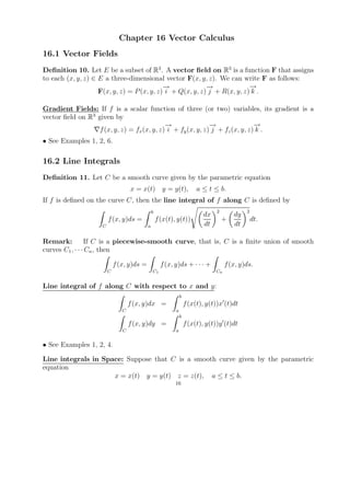
Download to read offline

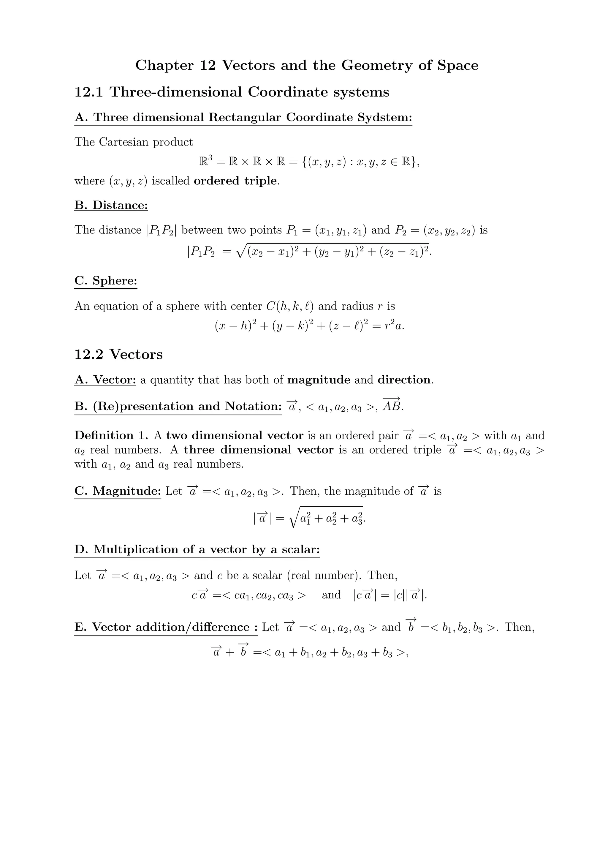
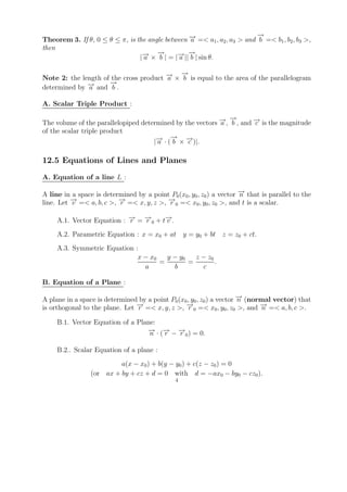
![13.2 Derivatives and Integrals of Vector Functions
A. Derivative : The derivative of a vector (valued) function − is defined by
→
r
d−
→r →
− (t + h) − − (t)
r →
r
= − (t) = lim
→
r
dt h→0 h
if the limit exists.
The vector − (t) is called the tangent vector of − , and it unit tangent vector is given
→
r →r
by
→
− (t)
r
T(t) = − → (t)| .
|r
Theorem 4. If r→
− (t) =< f (t), g(t), h(t) >, where f , g, and h are differentiable functions,
then
→
− (t) =< f (t), g (t), h (t) > .
r
Theorem 5. Suppose − and − are differentiable vector functions, c is a scalar, and f is
→
u →
v
a real valued function. Then,
d −
(1) [→(t) + − (t)] = − (t) + − (t)
u →v →u →
v
dt
d −
(2) [c→(t)] = c− (t)
u →u
dt
d
(3) [f (t)− (t)] = f (t)− (t) + f (t)− (t)
→
u →u →
u
dt
d −
(4) [→(t) · − (t)] = − (t) · − (t) + − (t) · − (t)
u →v →
u →v →u →
v
dt
d −
(5) [→(t) × − (t)] = − (t) × − (t) + − (t) × − (t)
u →v →u →
v →
u →
v
dt
d −
(6) [→(f (t))] = f (t)− (f (t)) (Chain Rule)
u →u
dt
• See Example 1-5
B. Integrals : If − (t) =< f (t), g(t), h(t) >, where f , g, and h are integrable in [a, b], then
→r
the definite integral if the vector function − (t) can be defined by
→
r
b b b b
→
− (t)dt = →
− →
− →
−
r f (t)dt i + g(t)dt j + h(t)dt k.
a a a a
• See Example 6
6](https://image.slidesharecdn.com/summarychapter1-chapter6-121204001219-phpapp01/85/Summary-chapter-1-chapter6-6-320.jpg)
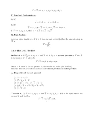
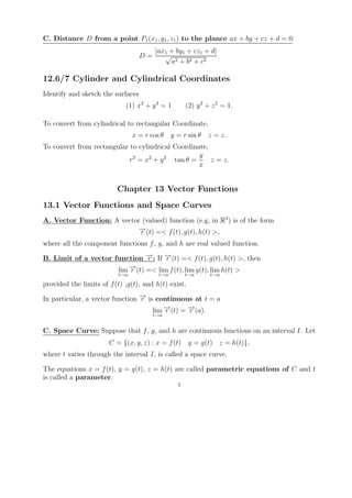
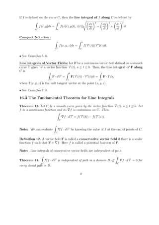
![13.3 Arc Length and Curvature
A. Arc Length : Let a ≤ t ≤ b, and let − (t) =< f (t), g(t), h(t) > where f , g , and h
→
r
are continuous on I. Then, the length of the space curve (arc length) from t = a to t = b
is defined by
b
L = →
− (t) 2 dt
r
a
b
= [f (t)]2 + [g (t)]2 + [h (t)]2 dt
a
b 2 2 2
dx dy dz
= + + dt
a dt dt dt
• See Example 1.
13.4 Motion in Space :Velocity and Acceleration
A. Velocity vector : Suppose a particle moves through space so that its position vector
at time t is − (t). The the velocity vector at time t is defined by
→
r
→
− →
−
− (t) = lim r (t + h) − r (t) = − (t).
→v →r
h→0 h
The velocity vector − (t) is also the tangent vector and points in the direction of the tangent
→v
line. Further, the speed of the particle at time t is
→
− (t) = − (t) .
v →r
B. Acceleration vector : The acceleration of the particle at time t is
→
− (t) = − (t) = − (t).
a →
v →r
• See Examples 1-3.
C. Newton’s Second Law of Motion : If, at any time t, a force F(t) acts on an object
of mass m producing an acceleration − (t), then
→
a
F(t) = m− (t).
→
a
• See Examples 4 and 5.
7](https://image.slidesharecdn.com/summarychapter1-chapter6-121204001219-phpapp01/85/Summary-chapter-1-chapter6-7-320.jpg)
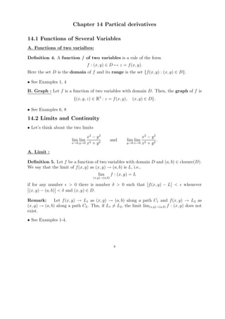
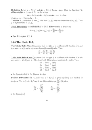
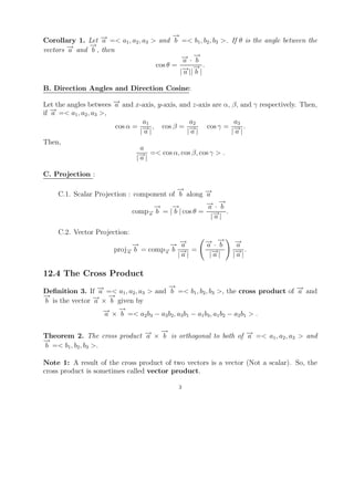
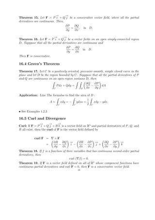
![14.6 Directional Derivatives and the Gradient Vector
A. Definition : Let f be a function of two variables. The directional derivatives of
f (x0 , y0 ) in the direction of unit vector − =< a, b > is
→
u
f (x0 + ha, y + hb) − f (x0 , y0 )
D− f (x0 , y0 ) = lim
→
u
h→0 h
if the limit exists.
In the case of three variable function, we can define the directional derivatives in a similar
manner.
Theorem 8. Let f be a differentialbe function of x and y. Then f has directional deriva-
tives in the direction of unit vector − =< a, b > and
→
u
D− f (x, y) = fx (x, y)a + fy (x, y)b.
→
u
The Gradient Vector : Let f be a function of several (say three) variables. The Gradient
of f is the vector function f fdefined by
→ ∂f − ∂f −
∂f − → →
f (x, y, z) =< fx (x, y, z), fy (x, y, z), fz (x, y, z) >= i + j k
∂x ∂x ∂z
Note that for any − =< a, b, c >, D− f (x, y, z) =
→
u →
u f (x, y, z) · − .
→
u
• See Examples 2, 3, 4
14.7 Maximum and Minimum Values
Definition 8. Let f be a function of two variables. Then, f (a, b) is called local maximum
value if f (a, b) ≥ f (x, y) when (x, y) is near (a, b). Also, f (a, b) is called local minimum
value if f (a, b) ≤ f (x, y) when (x, y) is near (a, b).
Theorem 9. If f has local maximum or minimum value at (a, b) and fx and fy exist, then
fx (a, b) = 0 and fy (a, b) = 0.
A point (a, b) is called a critical point of f if fx )a, b) = 0 and fy (a, b) = 0.
Second Derivatives Test: Assume that the second partial derivatives of f are continuous
on a disk with center (a, b), and assume that fx (a, b) = 0 and fy (a, b) = 0. Let
D = fxx (a, b)fyy (a, b) − [fxy (a, b)]2 .
(a) If D > 0 and fxx (a, b) > 0, then f (a, b) is a local minimum.
(b) If D > 0 and fxx (a, b) < 0, then f (a, b) is a local maximum.
11](https://image.slidesharecdn.com/summarychapter1-chapter6-121204001219-phpapp01/85/Summary-chapter-1-chapter6-11-320.jpg)
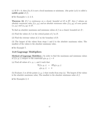
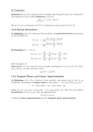
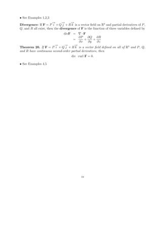
![Chapter 15 Multiple Integrals
15.1 Double Integrals over Rectangles
Definition 9. The double integral of f over R = [a, b] × [c, d] is
∞ ∞
f (x, y)dA = lim f (xi , yj )∆A (1)
R m,n→∞
i=1 j=1
if the limit exists, where (xi , yj ) is in
Rij = [xi−1 , xi ] × [yj−1 , yj ].
Here the right-hand side of (1) is called s double Riemann sum.
If f (x, y) ≥ 0, the volume V of the solid that lies above the rectangle R and below the
surface z = f (x, y) is
V = f (x, y)dA.
R
15.2 Iterated Integrals
Theorem 11. (Fubini) Let f be a continuous function on R = [a, b] × [c, d].
b d d b
f (x, y)dA = f (x, y)dydx = f (x, y)dxdy.
R a c c a
The two integrals in the right-hand side of the above identity are called iterated integrals.
More generally, this theorem is true if f is bounded on R, f is discontinuous only on a
finite number if snmooth curves, and the iterated integrals exist.
Special Cases : If f (x, y) = g(x)h(y) on R = [a, b] × [c, d],
b d d b
f (x, y)dA = f (x, y)dydx = h(y)dy · g(x)dx .
R a c c a
• See Examples 1-5.
15.3 Double Integrals over General Regions
Type I : Let f be a continuous on a type I region D such that
D = {(x, y)|a ≤ x ≤ b, g1 (x) ≤ y ≤ g2 (x)}
then
b g2 (x)
f (x, y)dA = f (x, y)dydx.
R a g1 (x)
13](https://image.slidesharecdn.com/summarychapter1-chapter6-121204001219-phpapp01/85/Summary-chapter-1-chapter6-13-320.jpg)
![Type II : Let f be a continuous on a type II region D such that
D = {(x, y)|c ≤ y ≤ d, h1 (x) ≤ x ≤ h2 (x)}
then
d h2 (x)
f (x, y)dA = f (x, y)dxdy.
R c h1 (x)
• See Examples 1-5.
Properties of Double Integrals : Assume that all of the following integrals exist. Then,
(1) [f (x, y) + g(x, y)]dA = f (x, y)dA + [g(x, y)]dA
D D D
(2) cf (x, y)dA = c [f (x, y)]dA
D D
(3) f (x, y)dA ≥ [g(x, y)]dA, if f (x, y) ≥ g(x, y)
D D
(4) 1dA = A(D)
D
(4) f (x, y)dA ≥ [g(x, y)]dA, + [g(x, y)]dA, if D = D1 ∪ D2 .
D D1 D2
Here D1 and D2 don’t overlap except (perhaps) on the boundary. Also, if m ≤ f (x, y) ≤ M
for all (x, y) ∈ D, then
mA(D) f (x, y)dA ≤ M A(D).
D
15.4 Double Integrals over Polar Coordinates
Change to Polar Coordinates in a Double Integral : Let f be a continuous on a po-
lar rectangle
R = {(r, θ) | 0 ≤ a ≤ r ≤ b, α ≤ θ ≤ β}
then
β b
f (x, y)dA = f (r cos θ, r sin θ)rdrdθ).
R α a
• See Examples 1,2.
15.7 Triple Integrals
14](https://image.slidesharecdn.com/summarychapter1-chapter6-121204001219-phpapp01/85/Summary-chapter-1-chapter6-14-320.jpg)
![Theorem 12. (Fubini’s Theorem for Triple Integrals) Let f be a continuous function on
B = [a, b] × [c, d] × [r, s].
s d b d b
f (x, y, z)dV = f (x, y, z)dxdydz = f (x, y)dxdy.
B r c a c a
Triple Integrals over General Regions:
Type I : Let f be a continuous on region D (type I or type II in double integral) such
that
E = {(x, y, z) | (x, y) ∈ D u1 (x, y) ≤ z ≤ u2 (x, y)},
then
u2 (x,y)
f (x, y, z)dV = f (x, y, z)dz dA.
E D u1 (x,y)
Type II : Let f be a continuous on region D (type I or type II in double integral) such
that
E = {(x, y, z) | (y, z) ∈ D u1 (y, z) ≤ z ≤ u2 (y, z)},
then
u2 (y,z)
f (x, y, z)dV = f (x, y, z)dx dA.
E D u1 (y,z)
• See Examples 1-3.
15.8 Triple Integrals in Cylindrical and Spherical Coordinates
Formula for triple integration in cylindrical coordinates:
u2 (r cos θ,r sin θ)
f (x, y, z)dV = f (r cos θ, r sin θ, z)rdzdrdθ.
E D u1 (r cos θ,r sin θ)
• See Examples 1,2.
15](https://image.slidesharecdn.com/summarychapter1-chapter6-121204001219-phpapp01/85/Summary-chapter-1-chapter6-15-320.jpg)

The document summarizes key concepts from a chapter on vectors and geometry in 3D space. [1] It introduces three-dimensional coordinate systems using ordered triples (x,y,z) and defines the distance formula between two points in 3D space. [2] It also defines concepts like the sphere equation and vectors, including their representation, magnitude, addition/subtraction, and dot and cross products. [3] It concludes by covering lines, planes, and their equations, as well as cylindrical coordinates.