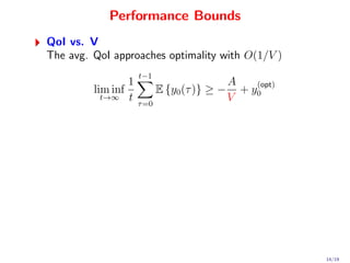
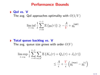
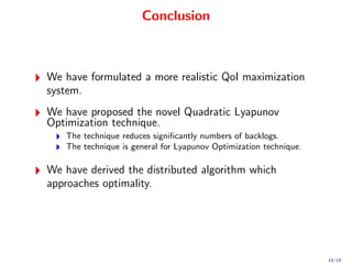
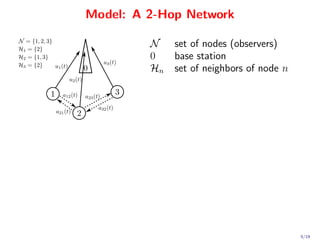
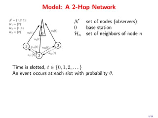
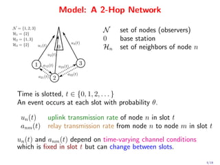
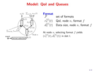
This document proposes a novel quadratic policy for maximizing quality of information (QoI) in a two-hop wireless network. It models a system where observers record random events in different formats, which have varying QoI values and data sizes. Data is transmitted over time-varying channels either directly or by relaying through neighbors, with a maximum of two hops. The policy formulates the problem using Lyapunov optimization to stabilize queues while maximizing average received QoI. It presents a quadratic formulation that yields separable subproblems allowing distributed implementation, improving over standard linearized approaches. Analysis shows average QoI achieves optimality within O(1/V) while average queue size grows within O(


![Lyapunov Drift Minimization
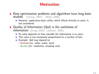
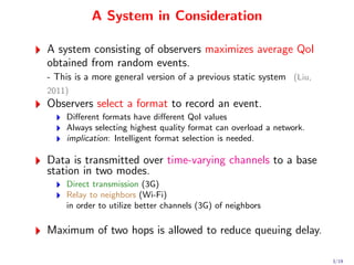
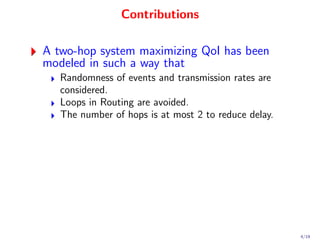
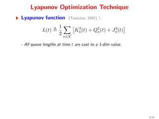
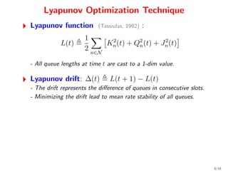
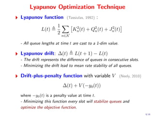
Pure Lyapunov optimization has quadratic nature of ∆(t).
1 2
min (max[Q(t) − b(t), 0] + a(t)) − Q2 (t)
a(t),b(t) 2
Reduce delay, Non-separable decisions (centralized algorithm)
10/19](https://image.slidesharecdn.com/icc2-120612124854-phpapp02/85/Sucha_ICC_2012-23-320.jpg)
![Lyapunov Drift Minimization
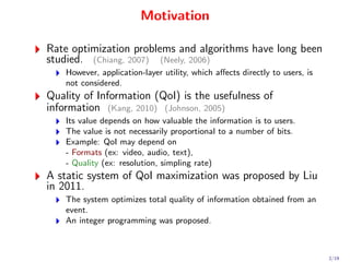
Pure Lyapunov optimization has quadratic nature of ∆(t).
1 2
min (max[Q(t) − b(t), 0] + a(t)) − Q2 (t)
a(t),b(t) 2
Reduce delay, Non-separable decisions (centralized algorithm)
Standard Lyapunov optimization optimizes a linearized ∆(t).
min Q(t) [a(t) − b(t)] (T assiulas, 1992)(N eely, 2010)
a(t),b(t)
Large delay, Separable decisions (distributed algorithm)
10/19](https://image.slidesharecdn.com/icc2-120612124854-phpapp02/85/Sucha_ICC_2012-24-320.jpg)
![Lyapunov Drift Minimization
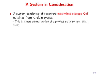
Pure Lyapunov optimization has quadratic nature of ∆(t).
1 2
min (max[Q(t) − b(t), 0] + a(t)) − Q2 (t)
a(t),b(t) 2
Reduce delay, Non-separable decisions (centralized algorithm)
Standard Lyapunov optimization optimizes a linearized ∆(t).
min Q(t) [a(t) − b(t)] (T assiulas, 1992)(N eely, 2010)
a(t),b(t)
Large delay, Separable decisions (distributed algorithm)
Novel Quadratic Lyapunov Optimization preserves the quadratic
nature of ∆(t).
2 2
min [Q(t) + a(t)] + [Q(t) − b(t)]
a(t),b(t)
Reduce delay, Separable decisions (distributed algorithm)
10/19](https://image.slidesharecdn.com/icc2-120612124854-phpapp02/85/Sucha_ICC_2012-25-320.jpg)
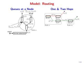
![Quadratic Policy
min
2 2
K (t) − s(q) (t) + K (t) − s(j) (t) +
n n
n n
2
(q)
[Kn (t) + dn (t)]2 + [Qn (t) − un (t)]2 + Qn (t) + sn (t) +
2 2
n∈N Qn (t) +
m∈Hn amn (t) + Jn (t) − m∈Hn anm (t) +
2
Jn (t) + s(j) (t) − 2V rn (t)
n
s. t.
s(q) (t) ∈ {0, 1, 2, . . . , s(q)(max) }, s(j) (t) ∈ {0, 1, 2, . . . , s(j)(max) } ,
n n n n
fn (t) ∈ F, dn (t) = d(fn (t)) (t), rn (t) = rn n (t)) (t) , n ∈ N
n
(f
a(t) ∈ Aγ(t) , u(t) ∈ Uγ(t)
11/19](https://image.slidesharecdn.com/icc2-120612124854-phpapp02/85/Sucha_ICC_2012-26-320.jpg)
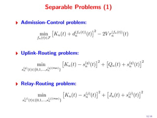
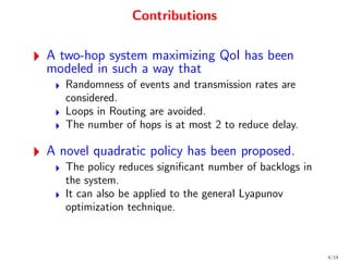
![Separable Problems (2)
Uplink-Allocation problem:
min [Qn (t) − un (t)]2
u(t)∈Uγ(t)
n∈N
Relay-Allocation problem:
2 2
min Qn (t) − amn (t) + Jn (t) − anm (t)
a(t)∈Aγ(t)
n∈N m∈Hn m∈Hn
13/19](https://image.slidesharecdn.com/icc2-120612124854-phpapp02/85/Sucha_ICC_2012-28-320.jpg)