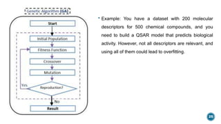
1
STATISTICAL
METHODS USED IN
QSAR
SUBMITTED BY
GOKUL K
1ST
M.PHARM
Dept. of Pharmaceutical Chemistry
SUBMITTED TO
Dr. SATISH N K
Dept. of Pharmaceutical Chemistry
COMPUTER AIDED DRUG DESIGN
SEMINAR ON
2
INTRODUCTION
 Quantitative structure–activity relationship (QSAR) is a methodology to associate the
chemical arrangement of a molecule with its biochemical, physical, pharmaceutical,
biological, etc., effect.
 QSAR models are developed for computational drug design, activity prediction, and
toxicology predictions.
 QSAR attempts to correlate structural, chemical, statistical, and physical properties with
biological potency using various mathematical methods.
 The generated QSAR models are used to predict and classify the biological activities of
new chemical compounds.
3
Requirements to generate a good quantitative
structure–activity relationship model
1. A set of molecules to be used for generating the QSAR model
2. A set of molecular descriptors generated for the data set of molecules
3. Biological activity (IC50, EC50, etc.) of the set of molecules
4. Statistical methods to develop a QSAR model
4
Statistical Methods
 Statistics is a branch of mathematics dealing with data collection, organization, analysis,
interpretation and presentation.
 Statistical method are mathematical formula, model and technique that are used in statistical
analysis of research data.
 Statistical methods are the mathematical foundation for the development of QSAR models.
 Statistical tools used for data pre-treatment feature selection, model development, validation
of QSAR. Multivariate statistical methods are needed to understand of multidimensional
data in its entirety.
5
Types of Statistical methods
6. Cluster analysis
7. Generic algorithm
8. Cross validation
9. Neuronal algorithm
1. Linear regression
2. Non linear regression
3. Principal component analysis
4. Partial least square regression
5. Support vector machine
6
Regression analysis
 Regression analysis is a statistical method used to model and analyse the relationships between a
dependent variable and one or more independent variables. The goal is to understand the relationship
between variables and to make predictions.
 If two variables are involved, the variable that is basis of estimation is called the independent variable and
the variable whose value is to be estimated is called as dependent variable.
 A dependent variable is a variable whose value depends upon independent variables. The dependent
variable is what being measured in an experiment or evaluated in a mathematical equation. The
dependent variable is sometimes called "The outcome variable”
 A independent variable is a variable that stands alone and isn't changed by the other variables you are
trying to measure.
7
1. Linear regression
 Linear regression is one of the simplest and most commonly used statistical methods in QSAR. It models the
relationship between a dependent variable (e.g., biological activity) and one independent variables
(descriptors, such as molecular weight, hydrophobicity, etc.). The relationship is assumed to be linear.
 Linear regression formula
Υ = β0+β1X+E
Where,
Υ = Dependent variable
β0 = Population Y intercept
β1 = Population slope coefficient
X = Independent variable
E = Random error
8
 Example: Suppose you have a dataset of chemical compounds with their biological
activity (e.g., IC50 values) and molecular descriptors like molecular weight (MW) and
logP (a measure of lipophilicity).
 The linear regression model could be:
9
2.Multiple Linear Regression (MLR)
 MLR is an extension of linear regression that involves multiple independent variables
(descriptors). It's commonly used in QSAR to model the effect of several molecular properties
on the activity of compounds.
 This model provides more accurate and precise results for complex substances.
 It is given by formula
Υ = β0+β1X1 + β2X2……………………….. βnXn +E
where n = number of variables
10
 Example: If you want to predict the toxicity of a set of compounds, you might use descriptors
like molecular volume, surface area, and electronegativity. The MLR model might look like:
Toxicity=β 0​+β 1​×Volume+β 2​×Surface Area+β 3​×Electronegativity+ϵ
11
3. Principal component analysis
 PCA is a dimensionality reduction technique that transforms a large set of descriptors into a
smaller set of uncorrelated variables called principal components.
 These components capture the most variance in the data, making it easier to visualize and
interpret the relationship between structure and activity.
 PCA is a technique of identifying patterns in data, and expressing data in such a way as to
emphasize their similarities and differences. It is also likely to be the oldest and the most
popular method in multivariate analysis.
12
 PCA is a useful data compression technique, by reducing the number of dimensions, without much
loss of information that has found applications in fields such as outlier detection, regression and is a
common technique for finding patterns in data of high dimension.
Example: If you have 100 molecular descriptors,
PCA can reduce this to a smaller number of principal components that still capture the majority of the
variance in the dataset. For example, you might reduce 100 descriptors to 3 principal components,
which can then be used in a regression model.
13
14
 Advantages of PCA in QSAR:
• Efficiency: PCA reduces computational complexity by shrinking the number of descriptors without
sacrificing much predictive power.
• Improves Model Generalization: By reducing the dimensionality, PCA helps prevent overfitting,
leading to better generalization of the QSAR model.
• Interpretability: While individual descriptors may be difficult to interpret, the principal components
represent combinations of descriptors that capture the most important variations in the data.
 Disadvantages of PCA:
• Loss of Interpretability: The principal components are linear combinations of the original
descriptors, which can make it harder to interpret their physical or chemical meaning in the context
of QSAR.
• Linear Method: PCA only captures linear relationships between descriptors, which may not be
sufficient for more complex datasets that exhibit non-linear relationships.
15
4.Partial least square regression
 Partial least square analysis (PLS) is a method for constructing predictive models when
the factors are many and collinear.
 It is a recent technique that generalizes and combines features from principal component
analysis and multiple regression
 PLS is particularly useful in QSAR when dealing with datasets with many highly correlated
descriptors. PLS finds the components (latent variables) that both explain the variance in
the descriptors and correlate with the activity.
16
 Partial Least Squares (PLS) regression is a powerful statistical method used in QSAR when there are
many highly correlated molecular descriptors (independent variables) and a relatively small number of
compounds (observations).
 PLS is particularly useful when dealing with multicollinearity—when descriptors are highly correlated
with each other, making traditional methods like Multiple Linear Regression (MLR) less effective.
 Example – if we want to predict the biological activity (e.g., IC50 values) of a set of chemical
compounds based on 30 molecular descriptors and some of these descriptors are highly correlated
with one another (e.g., different measures of molecular size), which makes linear regression ineffective
due to multicollinearity.
 We apply PLS to this data set and extract 5 latent variables that explains 80% of the variance in both
descriptor and biological activity.
 Using this 5 variables we build regression model to predict the lC50 value
17
 Advantages of PLS in QSAR:
• Handles Multicollinearity: PLS can handle highly correlated descriptors, which often
occur in QSAR datasets.
• Dimension Reduction: It reduces the number of variables by creating new latent
variables that explain most of the variance.
• Predicts Activity: PLS focuses on maximizing the covariance between descriptors and
biological activity, improving prediction quality.
• Improves Interpretation: While latent variables may not be directly interpretable like
individual descriptors, PLS helps uncover the underlying structure of the relationship
between structure and activity
18
5.Support Vector Machines
(SVM)
 Support Vector Machines (SVM) is a powerful machine learning method
used in QSAR modeling, particularly when dealing with complex, nonlinear
relationships between molecular descriptors (independent variables) and
biological activity (dependent variable). SVMs are widely used for
classification and regression tasks in QSAR, making them suitable for both
classifying compounds (e.g., active vs. inactive) and predicting continuous
outcomes (e.g., IC50 values).
19
 SVM works by finding the optimal boundary (called a hyperplane) that best separates data
points into different classes (for classification) or that best predicts continuous outcomes (for
regression). SVMs can handle both linear and nonlinear data, making them versatile for
QSAR models.
 Kernel Trick:
In many QSAR datasets, the relationship between molecular descriptors and activity is
nonlinear. SVM uses kernels to transform the data into a higher-dimensional space where a
linear boundary (hyperplane) can be created to separate or predict the data. The most common
kernels include:
• Linear Kernel: Used when the data is linearly separable.
• Polynomial Kernel: Captures polynomial relationships between variables.
• Radial Basis Function (RBF) Kernel: Commonly used in QSAR for capturing complex, nonlinear
relationships.
20
 Example: Linear Kernel in QSAR
While predicting whether a set of small-molecule inhibitors are active or inactive against a
particular protein target. It has molecular descriptors (e.g., molecular weight, logP, hydrogen bond
donors, etc.) for each compound. SVM with a linear kernel if the relationship between these
molecular descriptors and activity is linear.
Example: in a dataset of 300 molecules, each described by 20 molecular descriptors, and their
inhibition constants (IC50 values) against a specific enzyme. The relationship between these
molecular descriptors and biological activity appears curved, suggesting that a linear model might
not be enough to capture the pattern. Then we use polynomial kernel.
21
 Advantages of SVM in QSAR:
• Handles Nonlinear Data: SVM is highly effective when there are nonlinear relationships
between descriptors and biological activity, thanks to the use of kernel functions.
• Robust to Overfitting: The regularization parameter C helps control the trade-off between fitting
the data perfectly and keeping the model generalizable to new data.
• Works Well with Small Datasets: SVM is particularly effective in QSAR models when the
number of compounds is small relative to the number of descriptors.
• Versatile: SVM can be used for both classification and regression tasks in QSAR, making it
applicable to a wide range of problems.
 Disadvantages of SVM in QSAR:
• Computationally Intensive: SVM, especially with nonlinear kernels, can be slow for large
datasets.
• Less Interpretable: Unlike linear regression models, SVM models (especially those with
nonlinear kernels) are harder to interpret in terms of which molecular descriptors contribute most
to the predictions.
22
6. Cluster analysis
 Cluster analysis is a statistical method used to group similar objects (in this case, chemical
compounds) into clusters based on their characteristics. In QSAR (Quantitative Structure-
Activity Relationship), cluster analysis is used to identify groups of compounds that share
similar structural or chemical properties and are likely to exhibit similar biological activities.
This technique is essential for reducing the complexity of large datasets, identifying patterns,
and guiding drug discovery and design.
23
Advantages of Cluster Analysis in QSAR:
• Simplifies Complex Datasets: By grouping similar compounds, cluster analysis reduces the
complexity of large QSAR datasets.
• Enhances Interpretability: Clusters provide a more interpretable view of the chemical
space, making it easier to identify patterns and relationships.
• Identifies New Leads: Clustering can reveal new groups of active compounds, leading to the
discovery of novel chemical scaffolds.
• Supports Data-Driven Decision Making: Clustering informs decisions on which compounds
to prioritize for further study based on their groupings.
Disadvantages:
• Choice of Parameters: The results of cluster analysis can be sensitive to the choice of
clustering algorithm, distance metric, and the number of clusters (in methods like K-means).
• Interpretation: Clusters may not always correspond to meaningful chemical or biological
categories, leading to potential misinterpretations.
• Computationally Intensive: For very large datasets, cluster analysis can be computationally
expensive, especially when dealing with high-dimensional data
24
7.Generic algorithm
 Genetic Algorithms (GAs) are a class of optimization algorithms inspired by the principles of
natural selection and genetics. In the context of QSAR (Quantitative Structure-Activity
Relationship), GAs are employed to optimize models, select molecular descriptors, and
explore chemical space effectively, particularly when dealing with complex and high-
dimensional data.
25
 Example: You have a dataset with 200 molecular
descriptors for 500 chemical compounds, and you
need to build a QSAR model that predicts biological
activity. However, not all descriptors are relevant, and
using all of them could lead to overfitting.
26
Advantages of Genetic Algorithms in QSAR:
• Efficient Search: GAs can explore a large solution space effectively, making them ideal for
problems with many variables, such as descriptor selection in QSAR.
• Avoidance of Local Optima: The stochastic nature of GAs helps avoid getting stuck in local
optima, potentially leading to better solutions.
• Flexibility: GAs can be adapted to optimize a wide range of QSAR problems, from descriptor
selection to compound design.
• Parallelism: GAs are inherently parallel, meaning different parts of the population can be
evaluated simultaneously, speeding up the optimization process.
Disadvantages:
• Computationally Intensive: GAs can require significant computational resources, especially
for large populations and complex fitness functions.
• Parameter Sensitivity: The performance of GAs can be sensitive to the choice of
parameters, such as population size, mutation rate, and crossover rate.
• Convergence Speed: GAs may converge slowly, especially if the fitness landscape is
complex or if the algorithm is not well-tuned.
27
8. Cross validation
 Cross-validation is a statistical technique used to assess the performance of predictive
models, such as those used in QSAR (Quantitative Structure-Activity Relationship)
studies. It is particularly important in QSAR because it helps ensure that the model is
generalizable and not overfitted to the specific dataset used for training.
 Overfitting occurs when a model is too complex and captures not only the underlying
trend in the data but also the noise. This results in a model that performs well on the
training data but poorly on unseen data.
 Cross-validation helps detect overfitting by evaluating the model on different subsets of
the data.
28
K-Fold Cross-Validation:
•Split your dataset of 100 compounds into 5 folds (K=5).
•Train the QSAR model on 4 folds and validate it on the remaining fold.
•Repeat the process 5 times, with each fold serving as the test set once.
•Calculate the average R² value across all 5 folds to estimate the model’s predictive power.
Leave-One-Out Cross-Validation:
•For more precise validation, perform LOOCV where each compound is left out once, and the
model is trained on the remaining 99 compounds. The model is then tested on the left-out
compound.
•Repeat this process 100 times (one for each compound) and average the results to get an
unbiased estimate of the model’s performance.
29
Advantages of Cross-Validation in QSAR:
• Prevents Overfitting: By testing the model on different subsets of data, cross-validation helps
detect overfitting and ensures that the model generalizes well to new data.
• Provides Robust Performance Estimates: Cross-validation gives a more reliable estimate of
model performance compared to a single train-test split.
• Facilitates Model Comparison: Different models or descriptor sets can be compared fairly
using cross-validation, helping to choose the best approach.
• Versatile: Cross-validation can be applied to any predictive model, from linear regression to
complex machine learning algorithms.
Disadvantages:
• Computationally Intensive: Cross-validation, especially with a large number of folds or
LOOCV, can be computationally demanding, especially for complex models or large datasets.
• Complexity: The results of cross-validation can be influenced by how the data is split, making
it important to carefully choose the method and ensure proper implementation.
30
9. Neuronal algorithm
 Neural Networks (NNs), often referred to as artificial neural networks (ANNs), are a class of
machine learning algorithms inspired by the structure and functioning of the human brain. In
QSAR (Quantitative Structure-Activity Relationship), neural networks are used to model complex
relationships between molecular structures (descriptors) and their biological activities. Due to
their ability to learn non-linear relationships, neural networks are particularly effective for handling
complex and high-dimensional data commonly encountered in QSAR studies
31
Advantages of Neural Networks in QSAR:
• Ability to Model Complex Relationships: Neural networks can learn non-linear relationships,
making them ideal for QSAR models where the relationship between structure and activity is
complex.
• Feature Learning: Neural networks can automatically learn relevant features from raw data,
potentially improving model performance without extensive feature engineering.
• Scalability: Neural networks can handle large datasets and high-dimensional data, which are
common in QSAR studies.
• Flexibility: Neural networks can be adapted to various QSAR tasks, from regression and
classification to multi-task learning.
Disadvantages:
• Computationally Intensive: Training neural networks, especially deep networks, can require
significant computational resources, particularly for large datasets.
• Risk of Overfitting: Neural networks, especially with many layers, can easily overfit, requiring
careful use of regularization techniques.
• Interpretability: Neural networks are often considered "black boxes" due to their complexity,
making it difficult to interpret how specific molecular features contribute to predictions.
32
References
 Bastikar V, Bastikar A, Gupta P. Quantitative structure–activity relationship-based
computational approaches. Computational Approaches for Novel Therapeutic and
Diagnostic Designing to Mitigate SARS-CoV-2 Infection. 2022:191–205. doi:
10.1016/B978-0-323-91172-6.00001-7. Epub 2022 Jul 15. PMCID: PMC9300454.
 Todeschini, R., Consonni, V. (2009). Molecular Descriptors for Chemoinformatics.
Wiley-VCH.
 Eriksson, L., Johansson, E., Kettaneh-Wold, N., Wold, S. (2001). Introduction to Multi-
and Megavariate Data Analysis Using Projection Methods (PCA & PLS). Umetrics.
33
Thank you

STATISTICAL METHODS USED IN QSAR- CADD MPHARM

  • 1.
    1 STATISTICAL METHODS USED IN QSAR SUBMITTEDBY GOKUL K 1ST M.PHARM Dept. of Pharmaceutical Chemistry SUBMITTED TO Dr. SATISH N K Dept. of Pharmaceutical Chemistry COMPUTER AIDED DRUG DESIGN SEMINAR ON
  • 2.
    2 INTRODUCTION  Quantitative structure–activityrelationship (QSAR) is a methodology to associate the chemical arrangement of a molecule with its biochemical, physical, pharmaceutical, biological, etc., effect.  QSAR models are developed for computational drug design, activity prediction, and toxicology predictions.  QSAR attempts to correlate structural, chemical, statistical, and physical properties with biological potency using various mathematical methods.  The generated QSAR models are used to predict and classify the biological activities of new chemical compounds.
  • 3.
    3 Requirements to generatea good quantitative structure–activity relationship model 1. A set of molecules to be used for generating the QSAR model 2. A set of molecular descriptors generated for the data set of molecules 3. Biological activity (IC50, EC50, etc.) of the set of molecules 4. Statistical methods to develop a QSAR model
  • 4.
    4 Statistical Methods  Statisticsis a branch of mathematics dealing with data collection, organization, analysis, interpretation and presentation.  Statistical method are mathematical formula, model and technique that are used in statistical analysis of research data.  Statistical methods are the mathematical foundation for the development of QSAR models.  Statistical tools used for data pre-treatment feature selection, model development, validation of QSAR. Multivariate statistical methods are needed to understand of multidimensional data in its entirety.
  • 5.
    5 Types of Statisticalmethods 6. Cluster analysis 7. Generic algorithm 8. Cross validation 9. Neuronal algorithm 1. Linear regression 2. Non linear regression 3. Principal component analysis 4. Partial least square regression 5. Support vector machine
  • 6.
    6 Regression analysis  Regressionanalysis is a statistical method used to model and analyse the relationships between a dependent variable and one or more independent variables. The goal is to understand the relationship between variables and to make predictions.  If two variables are involved, the variable that is basis of estimation is called the independent variable and the variable whose value is to be estimated is called as dependent variable.  A dependent variable is a variable whose value depends upon independent variables. The dependent variable is what being measured in an experiment or evaluated in a mathematical equation. The dependent variable is sometimes called "The outcome variable”  A independent variable is a variable that stands alone and isn't changed by the other variables you are trying to measure.
  • 7.
    7 1. Linear regression Linear regression is one of the simplest and most commonly used statistical methods in QSAR. It models the relationship between a dependent variable (e.g., biological activity) and one independent variables (descriptors, such as molecular weight, hydrophobicity, etc.). The relationship is assumed to be linear.  Linear regression formula Υ = β0+β1X+E Where, Υ = Dependent variable β0 = Population Y intercept β1 = Population slope coefficient X = Independent variable E = Random error
  • 8.
    8  Example: Supposeyou have a dataset of chemical compounds with their biological activity (e.g., IC50 values) and molecular descriptors like molecular weight (MW) and logP (a measure of lipophilicity).  The linear regression model could be:
  • 9.
    9 2.Multiple Linear Regression(MLR)  MLR is an extension of linear regression that involves multiple independent variables (descriptors). It's commonly used in QSAR to model the effect of several molecular properties on the activity of compounds.  This model provides more accurate and precise results for complex substances.  It is given by formula Υ = β0+β1X1 + β2X2……………………….. βnXn +E where n = number of variables
  • 10.
    10  Example: Ifyou want to predict the toxicity of a set of compounds, you might use descriptors like molecular volume, surface area, and electronegativity. The MLR model might look like: Toxicity=β 0​+β 1​×Volume+β 2​×Surface Area+β 3​×Electronegativity+ϵ
  • 11.
    11 3. Principal componentanalysis  PCA is a dimensionality reduction technique that transforms a large set of descriptors into a smaller set of uncorrelated variables called principal components.  These components capture the most variance in the data, making it easier to visualize and interpret the relationship between structure and activity.  PCA is a technique of identifying patterns in data, and expressing data in such a way as to emphasize their similarities and differences. It is also likely to be the oldest and the most popular method in multivariate analysis.
  • 12.
    12  PCA isa useful data compression technique, by reducing the number of dimensions, without much loss of information that has found applications in fields such as outlier detection, regression and is a common technique for finding patterns in data of high dimension. Example: If you have 100 molecular descriptors, PCA can reduce this to a smaller number of principal components that still capture the majority of the variance in the dataset. For example, you might reduce 100 descriptors to 3 principal components, which can then be used in a regression model.
  • 13.
  • 14.
    14  Advantages ofPCA in QSAR: • Efficiency: PCA reduces computational complexity by shrinking the number of descriptors without sacrificing much predictive power. • Improves Model Generalization: By reducing the dimensionality, PCA helps prevent overfitting, leading to better generalization of the QSAR model. • Interpretability: While individual descriptors may be difficult to interpret, the principal components represent combinations of descriptors that capture the most important variations in the data.  Disadvantages of PCA: • Loss of Interpretability: The principal components are linear combinations of the original descriptors, which can make it harder to interpret their physical or chemical meaning in the context of QSAR. • Linear Method: PCA only captures linear relationships between descriptors, which may not be sufficient for more complex datasets that exhibit non-linear relationships.
  • 15.
    15 4.Partial least squareregression  Partial least square analysis (PLS) is a method for constructing predictive models when the factors are many and collinear.  It is a recent technique that generalizes and combines features from principal component analysis and multiple regression  PLS is particularly useful in QSAR when dealing with datasets with many highly correlated descriptors. PLS finds the components (latent variables) that both explain the variance in the descriptors and correlate with the activity.
  • 16.
    16  Partial LeastSquares (PLS) regression is a powerful statistical method used in QSAR when there are many highly correlated molecular descriptors (independent variables) and a relatively small number of compounds (observations).  PLS is particularly useful when dealing with multicollinearity—when descriptors are highly correlated with each other, making traditional methods like Multiple Linear Regression (MLR) less effective.  Example – if we want to predict the biological activity (e.g., IC50 values) of a set of chemical compounds based on 30 molecular descriptors and some of these descriptors are highly correlated with one another (e.g., different measures of molecular size), which makes linear regression ineffective due to multicollinearity.  We apply PLS to this data set and extract 5 latent variables that explains 80% of the variance in both descriptor and biological activity.  Using this 5 variables we build regression model to predict the lC50 value
  • 17.
    17  Advantages ofPLS in QSAR: • Handles Multicollinearity: PLS can handle highly correlated descriptors, which often occur in QSAR datasets. • Dimension Reduction: It reduces the number of variables by creating new latent variables that explain most of the variance. • Predicts Activity: PLS focuses on maximizing the covariance between descriptors and biological activity, improving prediction quality. • Improves Interpretation: While latent variables may not be directly interpretable like individual descriptors, PLS helps uncover the underlying structure of the relationship between structure and activity
  • 18.
    18 5.Support Vector Machines (SVM) Support Vector Machines (SVM) is a powerful machine learning method used in QSAR modeling, particularly when dealing with complex, nonlinear relationships between molecular descriptors (independent variables) and biological activity (dependent variable). SVMs are widely used for classification and regression tasks in QSAR, making them suitable for both classifying compounds (e.g., active vs. inactive) and predicting continuous outcomes (e.g., IC50 values).
  • 19.
    19  SVM worksby finding the optimal boundary (called a hyperplane) that best separates data points into different classes (for classification) or that best predicts continuous outcomes (for regression). SVMs can handle both linear and nonlinear data, making them versatile for QSAR models.  Kernel Trick: In many QSAR datasets, the relationship between molecular descriptors and activity is nonlinear. SVM uses kernels to transform the data into a higher-dimensional space where a linear boundary (hyperplane) can be created to separate or predict the data. The most common kernels include: • Linear Kernel: Used when the data is linearly separable. • Polynomial Kernel: Captures polynomial relationships between variables. • Radial Basis Function (RBF) Kernel: Commonly used in QSAR for capturing complex, nonlinear relationships.
  • 20.
    20  Example: LinearKernel in QSAR While predicting whether a set of small-molecule inhibitors are active or inactive against a particular protein target. It has molecular descriptors (e.g., molecular weight, logP, hydrogen bond donors, etc.) for each compound. SVM with a linear kernel if the relationship between these molecular descriptors and activity is linear. Example: in a dataset of 300 molecules, each described by 20 molecular descriptors, and their inhibition constants (IC50 values) against a specific enzyme. The relationship between these molecular descriptors and biological activity appears curved, suggesting that a linear model might not be enough to capture the pattern. Then we use polynomial kernel.
  • 21.
    21  Advantages ofSVM in QSAR: • Handles Nonlinear Data: SVM is highly effective when there are nonlinear relationships between descriptors and biological activity, thanks to the use of kernel functions. • Robust to Overfitting: The regularization parameter C helps control the trade-off between fitting the data perfectly and keeping the model generalizable to new data. • Works Well with Small Datasets: SVM is particularly effective in QSAR models when the number of compounds is small relative to the number of descriptors. • Versatile: SVM can be used for both classification and regression tasks in QSAR, making it applicable to a wide range of problems.  Disadvantages of SVM in QSAR: • Computationally Intensive: SVM, especially with nonlinear kernels, can be slow for large datasets. • Less Interpretable: Unlike linear regression models, SVM models (especially those with nonlinear kernels) are harder to interpret in terms of which molecular descriptors contribute most to the predictions.
  • 22.
    22 6. Cluster analysis Cluster analysis is a statistical method used to group similar objects (in this case, chemical compounds) into clusters based on their characteristics. In QSAR (Quantitative Structure- Activity Relationship), cluster analysis is used to identify groups of compounds that share similar structural or chemical properties and are likely to exhibit similar biological activities. This technique is essential for reducing the complexity of large datasets, identifying patterns, and guiding drug discovery and design.
  • 23.
    23 Advantages of ClusterAnalysis in QSAR: • Simplifies Complex Datasets: By grouping similar compounds, cluster analysis reduces the complexity of large QSAR datasets. • Enhances Interpretability: Clusters provide a more interpretable view of the chemical space, making it easier to identify patterns and relationships. • Identifies New Leads: Clustering can reveal new groups of active compounds, leading to the discovery of novel chemical scaffolds. • Supports Data-Driven Decision Making: Clustering informs decisions on which compounds to prioritize for further study based on their groupings. Disadvantages: • Choice of Parameters: The results of cluster analysis can be sensitive to the choice of clustering algorithm, distance metric, and the number of clusters (in methods like K-means). • Interpretation: Clusters may not always correspond to meaningful chemical or biological categories, leading to potential misinterpretations. • Computationally Intensive: For very large datasets, cluster analysis can be computationally expensive, especially when dealing with high-dimensional data
  • 24.
    24 7.Generic algorithm  GeneticAlgorithms (GAs) are a class of optimization algorithms inspired by the principles of natural selection and genetics. In the context of QSAR (Quantitative Structure-Activity Relationship), GAs are employed to optimize models, select molecular descriptors, and explore chemical space effectively, particularly when dealing with complex and high- dimensional data.
  • 25.
    25  Example: Youhave a dataset with 200 molecular descriptors for 500 chemical compounds, and you need to build a QSAR model that predicts biological activity. However, not all descriptors are relevant, and using all of them could lead to overfitting.
  • 26.
    26 Advantages of GeneticAlgorithms in QSAR: • Efficient Search: GAs can explore a large solution space effectively, making them ideal for problems with many variables, such as descriptor selection in QSAR. • Avoidance of Local Optima: The stochastic nature of GAs helps avoid getting stuck in local optima, potentially leading to better solutions. • Flexibility: GAs can be adapted to optimize a wide range of QSAR problems, from descriptor selection to compound design. • Parallelism: GAs are inherently parallel, meaning different parts of the population can be evaluated simultaneously, speeding up the optimization process. Disadvantages: • Computationally Intensive: GAs can require significant computational resources, especially for large populations and complex fitness functions. • Parameter Sensitivity: The performance of GAs can be sensitive to the choice of parameters, such as population size, mutation rate, and crossover rate. • Convergence Speed: GAs may converge slowly, especially if the fitness landscape is complex or if the algorithm is not well-tuned.
  • 27.
    27 8. Cross validation Cross-validation is a statistical technique used to assess the performance of predictive models, such as those used in QSAR (Quantitative Structure-Activity Relationship) studies. It is particularly important in QSAR because it helps ensure that the model is generalizable and not overfitted to the specific dataset used for training.  Overfitting occurs when a model is too complex and captures not only the underlying trend in the data but also the noise. This results in a model that performs well on the training data but poorly on unseen data.  Cross-validation helps detect overfitting by evaluating the model on different subsets of the data.
  • 28.
    28 K-Fold Cross-Validation: •Split yourdataset of 100 compounds into 5 folds (K=5). •Train the QSAR model on 4 folds and validate it on the remaining fold. •Repeat the process 5 times, with each fold serving as the test set once. •Calculate the average R² value across all 5 folds to estimate the model’s predictive power. Leave-One-Out Cross-Validation: •For more precise validation, perform LOOCV where each compound is left out once, and the model is trained on the remaining 99 compounds. The model is then tested on the left-out compound. •Repeat this process 100 times (one for each compound) and average the results to get an unbiased estimate of the model’s performance.
  • 29.
    29 Advantages of Cross-Validationin QSAR: • Prevents Overfitting: By testing the model on different subsets of data, cross-validation helps detect overfitting and ensures that the model generalizes well to new data. • Provides Robust Performance Estimates: Cross-validation gives a more reliable estimate of model performance compared to a single train-test split. • Facilitates Model Comparison: Different models or descriptor sets can be compared fairly using cross-validation, helping to choose the best approach. • Versatile: Cross-validation can be applied to any predictive model, from linear regression to complex machine learning algorithms. Disadvantages: • Computationally Intensive: Cross-validation, especially with a large number of folds or LOOCV, can be computationally demanding, especially for complex models or large datasets. • Complexity: The results of cross-validation can be influenced by how the data is split, making it important to carefully choose the method and ensure proper implementation.
  • 30.
    30 9. Neuronal algorithm Neural Networks (NNs), often referred to as artificial neural networks (ANNs), are a class of machine learning algorithms inspired by the structure and functioning of the human brain. In QSAR (Quantitative Structure-Activity Relationship), neural networks are used to model complex relationships between molecular structures (descriptors) and their biological activities. Due to their ability to learn non-linear relationships, neural networks are particularly effective for handling complex and high-dimensional data commonly encountered in QSAR studies
  • 31.
    31 Advantages of NeuralNetworks in QSAR: • Ability to Model Complex Relationships: Neural networks can learn non-linear relationships, making them ideal for QSAR models where the relationship between structure and activity is complex. • Feature Learning: Neural networks can automatically learn relevant features from raw data, potentially improving model performance without extensive feature engineering. • Scalability: Neural networks can handle large datasets and high-dimensional data, which are common in QSAR studies. • Flexibility: Neural networks can be adapted to various QSAR tasks, from regression and classification to multi-task learning. Disadvantages: • Computationally Intensive: Training neural networks, especially deep networks, can require significant computational resources, particularly for large datasets. • Risk of Overfitting: Neural networks, especially with many layers, can easily overfit, requiring careful use of regularization techniques. • Interpretability: Neural networks are often considered "black boxes" due to their complexity, making it difficult to interpret how specific molecular features contribute to predictions.
  • 32.
    32 References  Bastikar V,Bastikar A, Gupta P. Quantitative structure–activity relationship-based computational approaches. Computational Approaches for Novel Therapeutic and Diagnostic Designing to Mitigate SARS-CoV-2 Infection. 2022:191–205. doi: 10.1016/B978-0-323-91172-6.00001-7. Epub 2022 Jul 15. PMCID: PMC9300454.  Todeschini, R., Consonni, V. (2009). Molecular Descriptors for Chemoinformatics. Wiley-VCH.  Eriksson, L., Johansson, E., Kettaneh-Wold, N., Wold, S. (2001). Introduction to Multi- and Megavariate Data Analysis Using Projection Methods (PCA & PLS). Umetrics.
  • 33.

Editor's Notes

  • #2 s also used as a screening and enrichment tool to remove the compounds and molecules that do not possess drug-likeness properties or are predicted toxic
  • #3 A dataset consisting of molecules, structurally similar, whose QSAR model needs to be developed are to be prepared for the QSAR study. Depending upon the type of QSAR the molecules need to be minimized or cleaned. Once the molecules are finalized, the parameters of the molecules known as the descriptors are calculated, which can be the overall structural properties of the molecules, two-dimensional properties of the molecules, three-dimensional properties of the molecule in space, or the different conformational properties of the molecules. The molecules whose QSAR model is to be developed should have a definite and known biological activity value that can be correlated with the molecular descriptors generated, to develop a good and reliable QSAR model. Various statistical methods like clustering, partial least square, regression, principal component analysis (PCA), etc., can be used to develop a mathematical correlation between the biological activity and the descriptors calculated.
  • #6 D- biological data I – physicochemical property
  • #11 PCA is a useful data compression technique, by reducing the number of dimensions, without much loss of information that has found applications in fields such as outlier detection, regression and is a common technique for finding patterns in data of high dimension.
  • #13 molecular weight, logP, polar surface area, et compute the Covariance Matrix -Instead of using all 50 descriptors, PCA selects a smaller number of principal components that explain most of the variance. For example, the first three principal components might explain 85% of the variance in the data.
  • #19 Support Vectors: These are the data points (compounds) that lie closest to the hyperplane. These points are crucial because they define the optimal boundary and ensure that the hyperplane maximizes the margin between classes.
  • #25 Population Initialization: Start with a population of random solutions, where each individual is a different subset of the 200 descriptors. Fitness Function: Define the fitness function as the predictive accuracy of a QSAR model (e.g., R² of a regression model or accuracy of a classification model) using the selected subset of descriptors. Selection: Select the top-performing individuals (e.g., those with the highest R² or classification accuracy) to act as parents for the next generation. Crossover and Mutation: Apply crossover to combine descriptor subsets from parent individuals and mutation to randomly include or exclude descriptors. This creates a new population of descriptor subsets. Generation of New Solutions: Evaluate the fitness of the new population and repeat the process for multiple generations, allowing the population to evolve toward better solutions. Termination: After a set number of generations or when the improvement plateaus, select the best-performing subset of descriptors as the final solution. Outcome: The GA will likely identify a subset of descriptors that provides a robust, predictive QSAR model with fewer features, reducing the risk of overfitting and improving interpretability.
  • #27 Cross-validation is essential for evaluating the predictive performance of QSAR models, ensuring that they are not just fitting the training data but can generalize to new, unseen compounds.
  • #30 nput Layer: The first layer that receives the input data (e.g., molecular descriptors).Hidden Layers: Intermediate layers where the network processes the inputs. Each hidden layer transforms the input through weighted connections and non-linear activation functions.Output Layer: The final layer that produces the prediction (e.g., biological activity of a compound). Weights are parameters that control the strength of the connection between neurons. During training, the network learns the optimal weights to minimize the error between predicted and actual outputs.Biases are additional parameters that shift the activation function, allowing the network to model complex patterns more effectively.