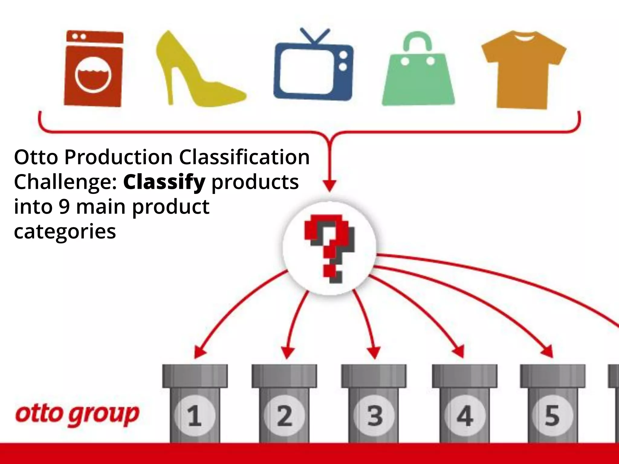
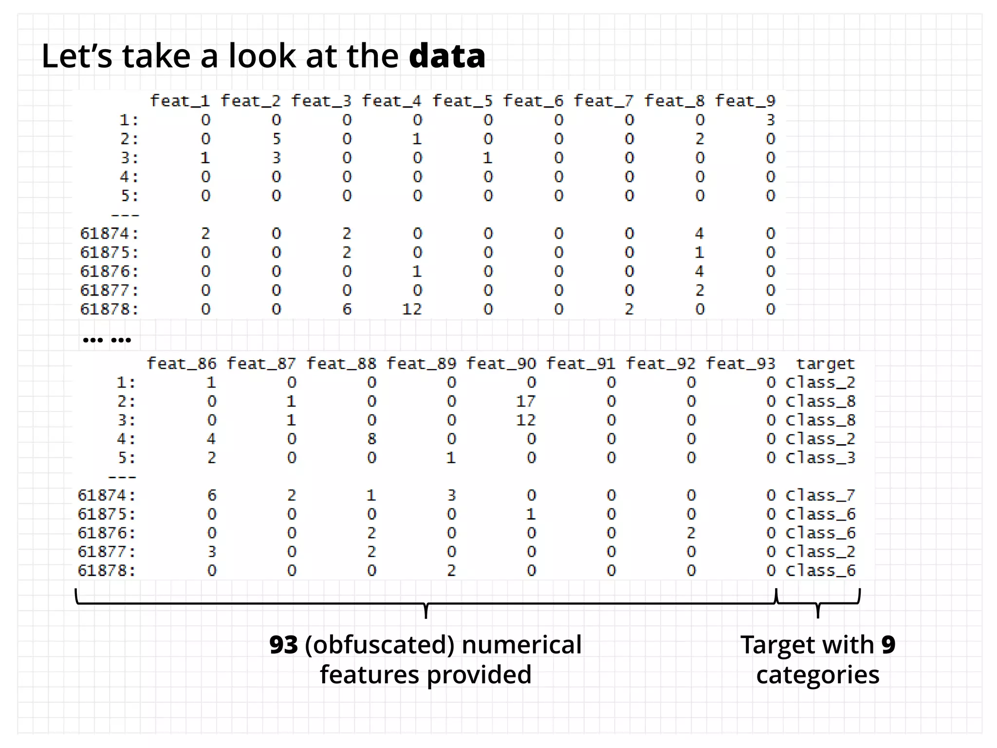
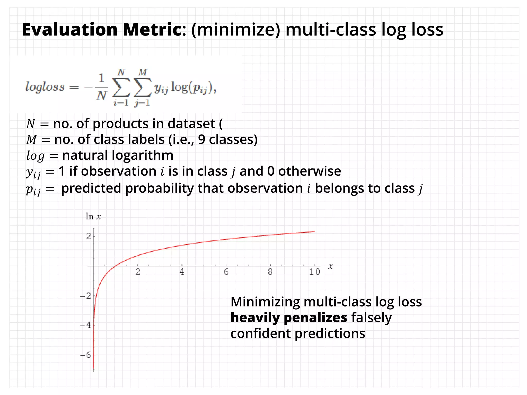
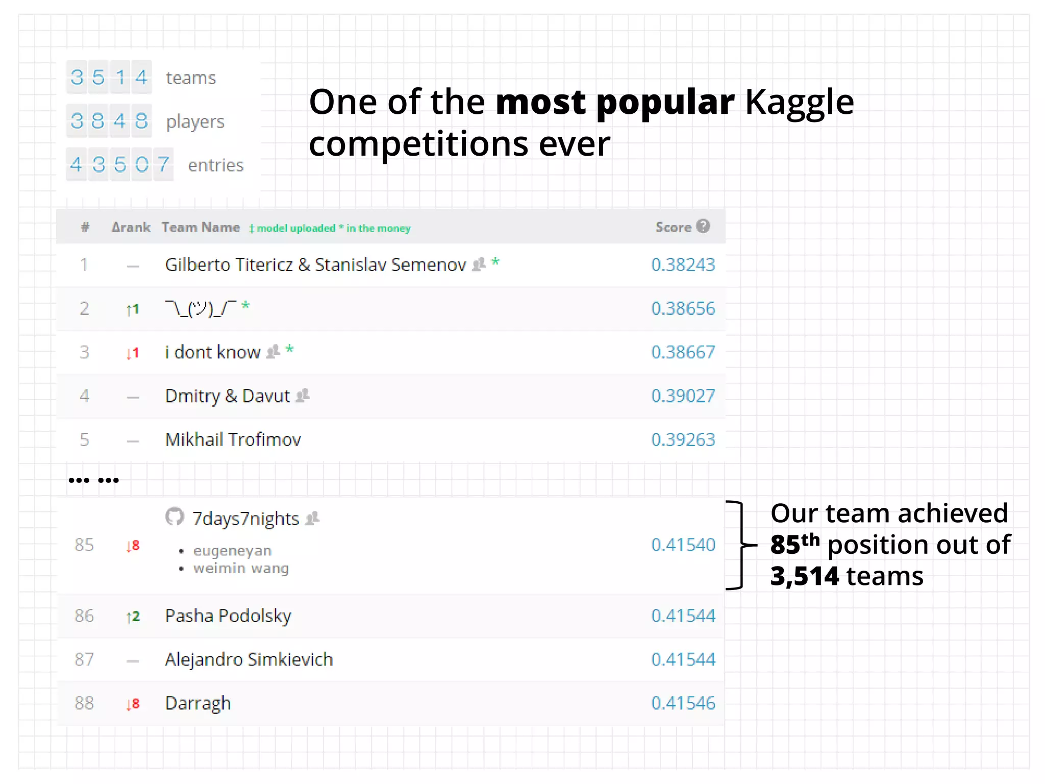
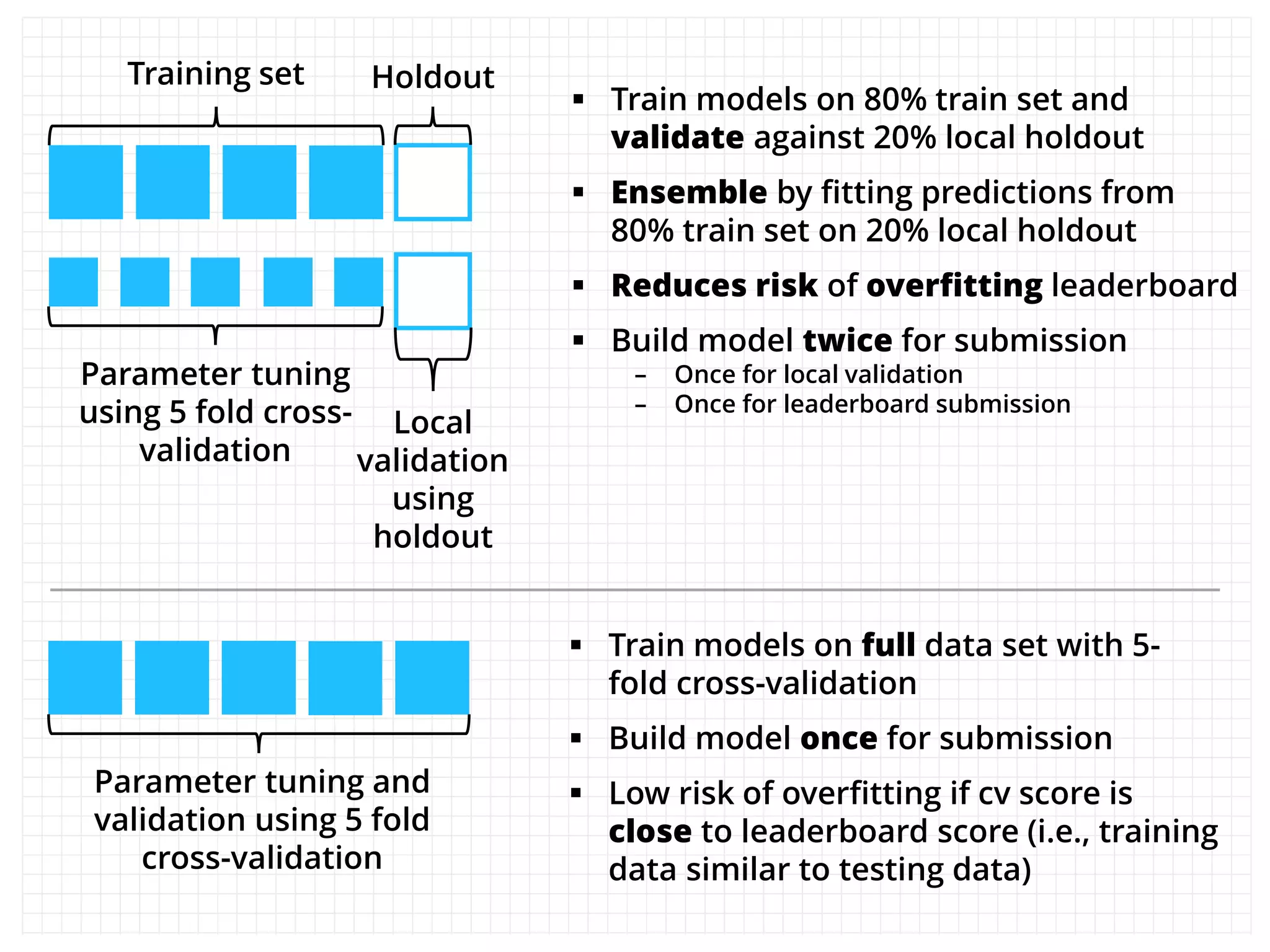
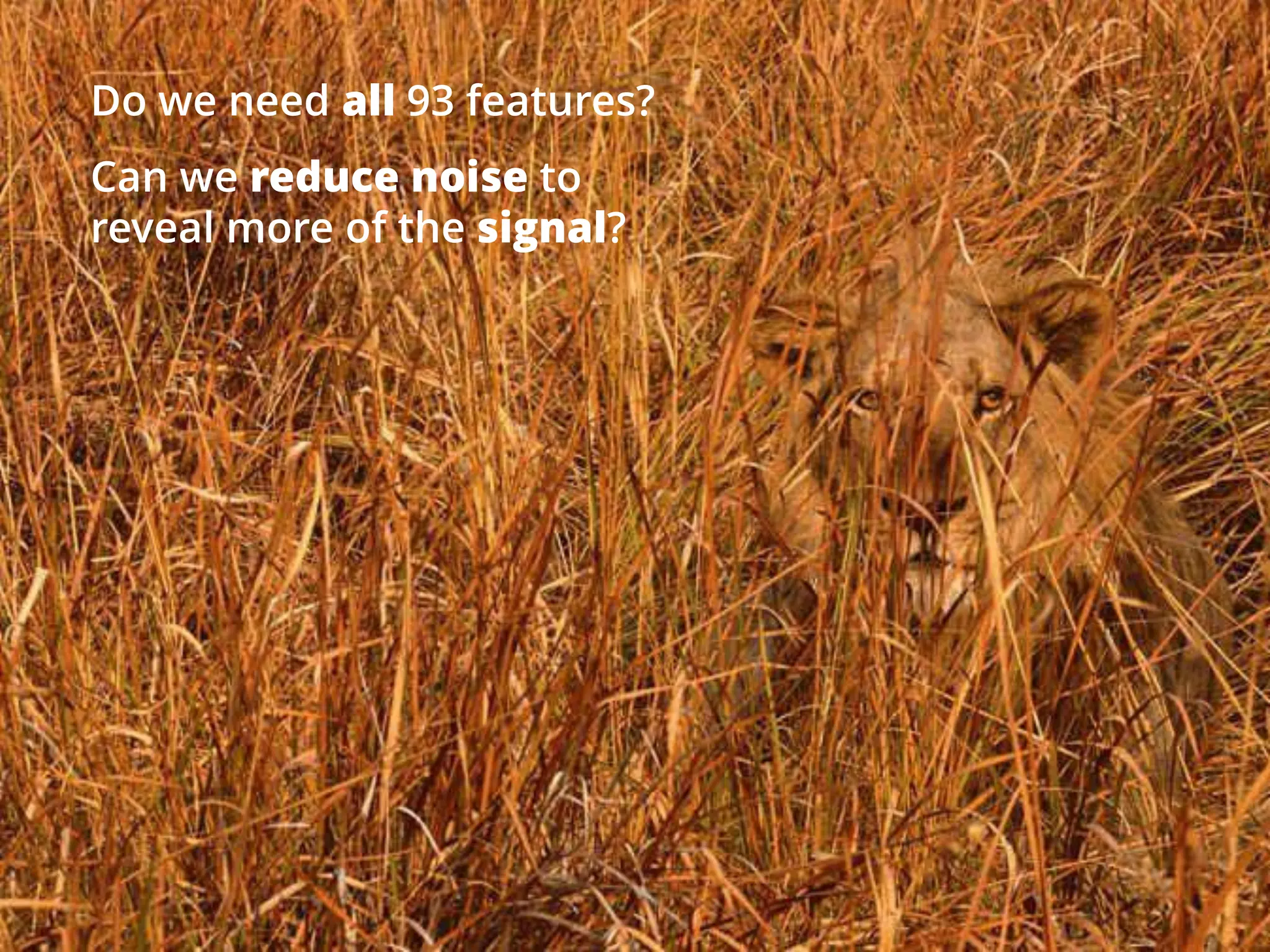
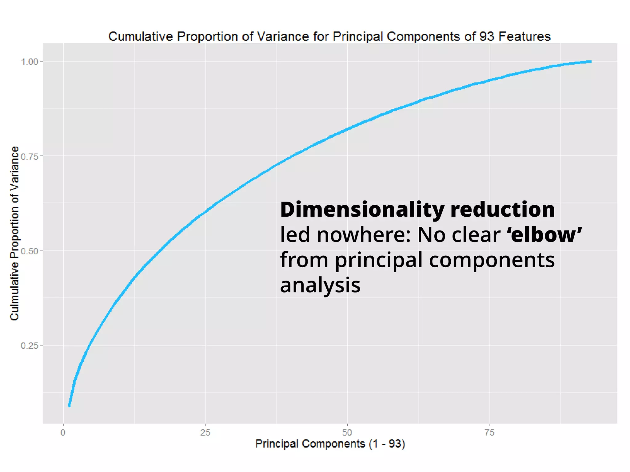
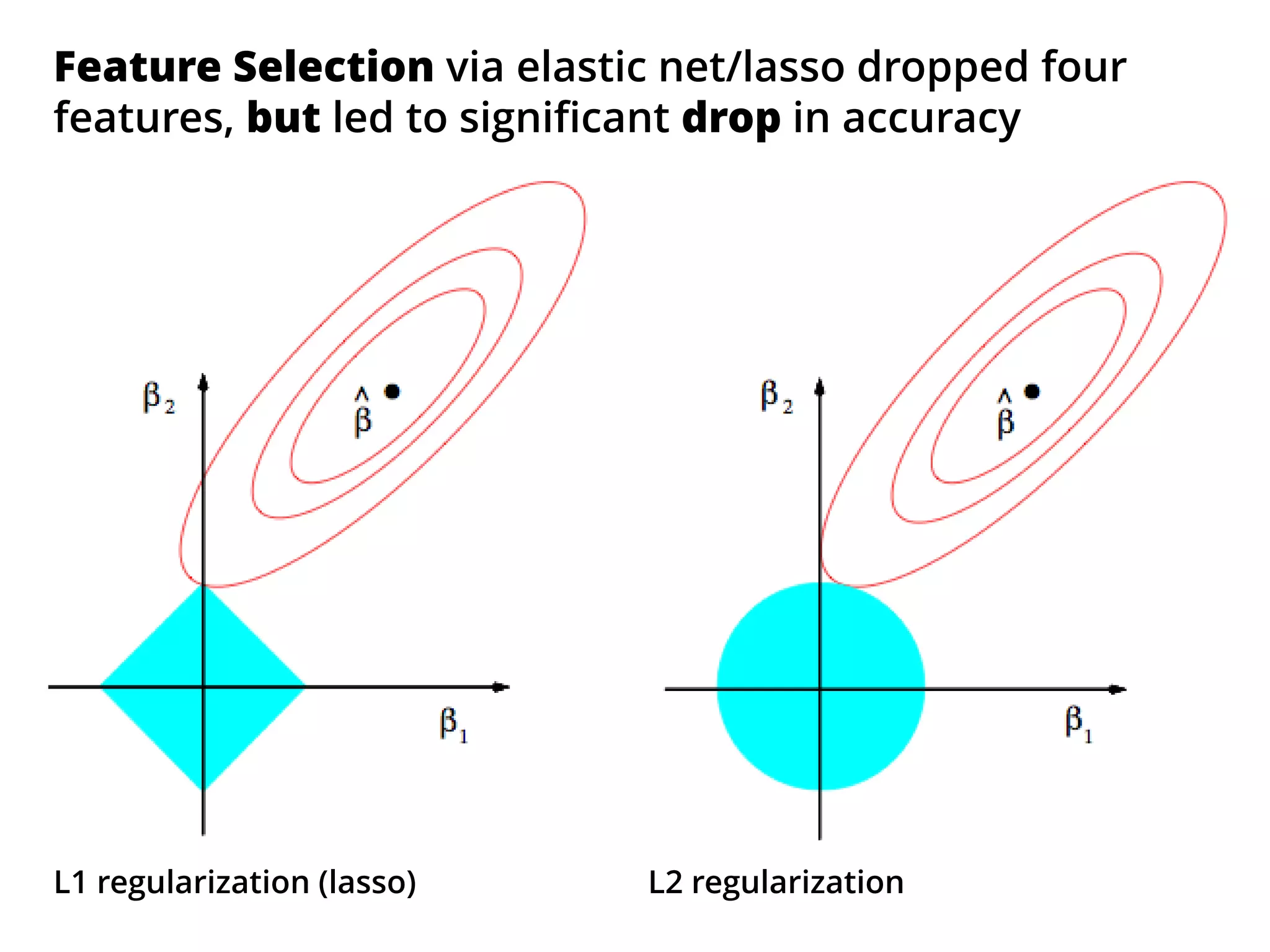
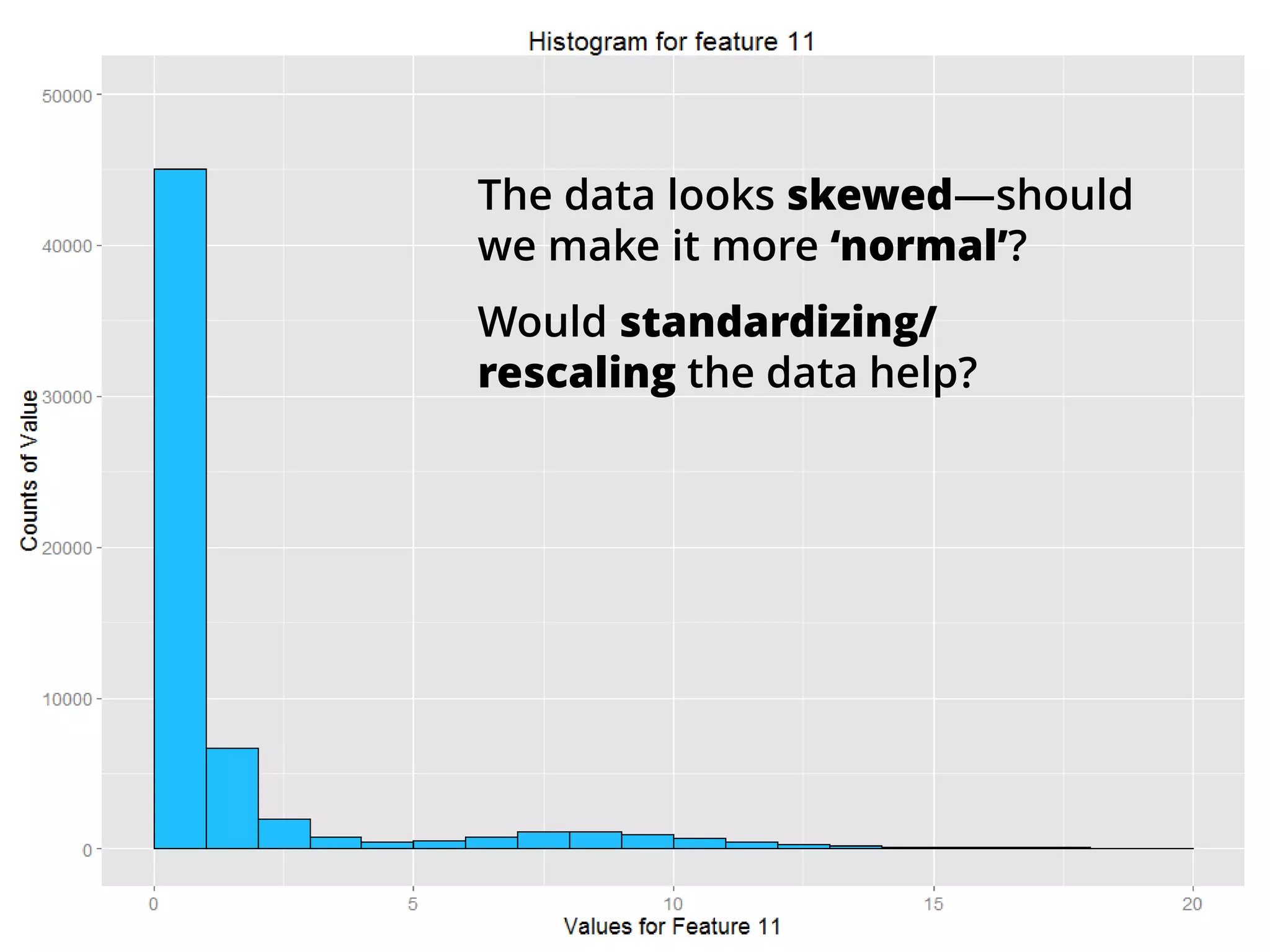
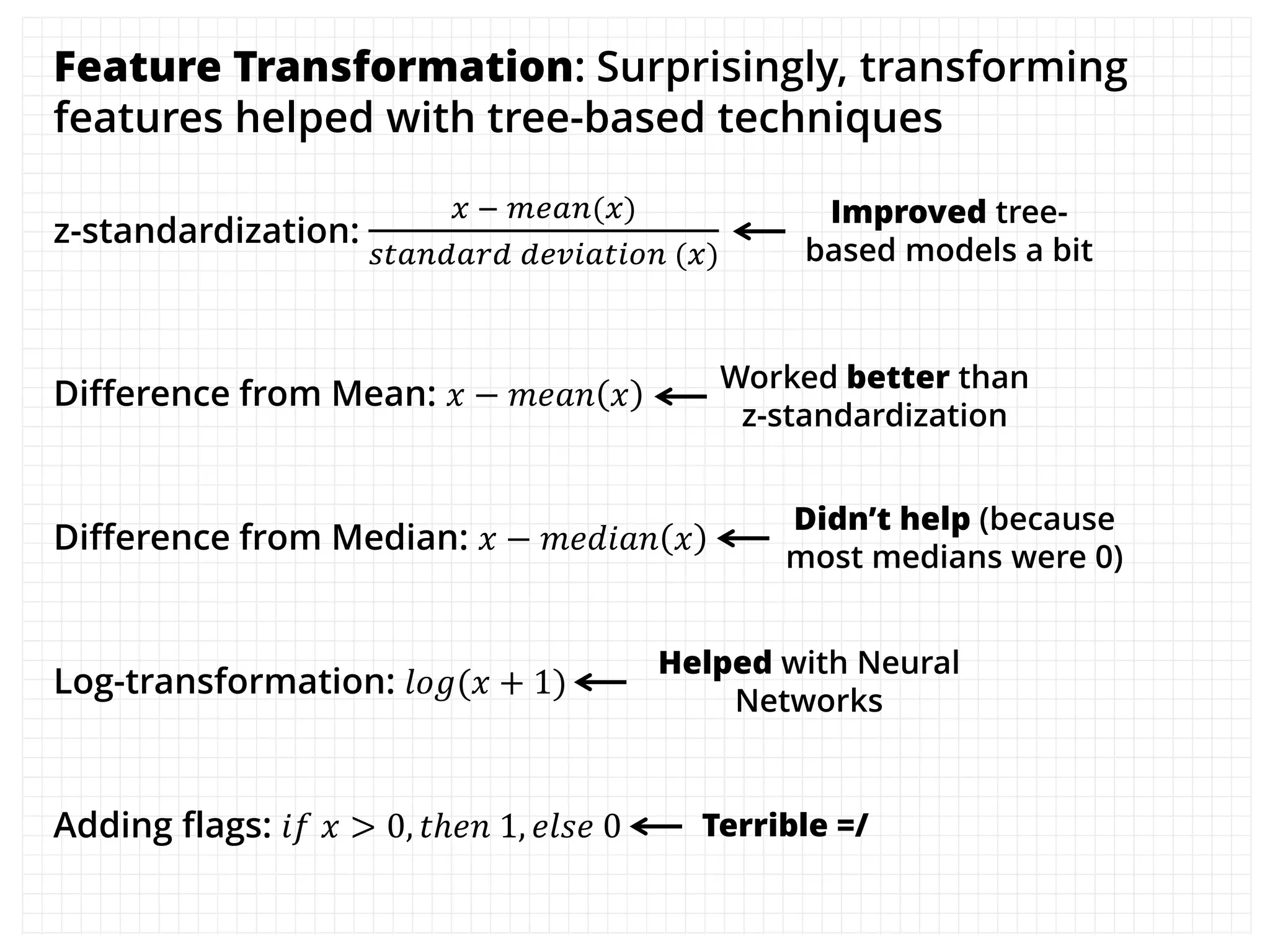
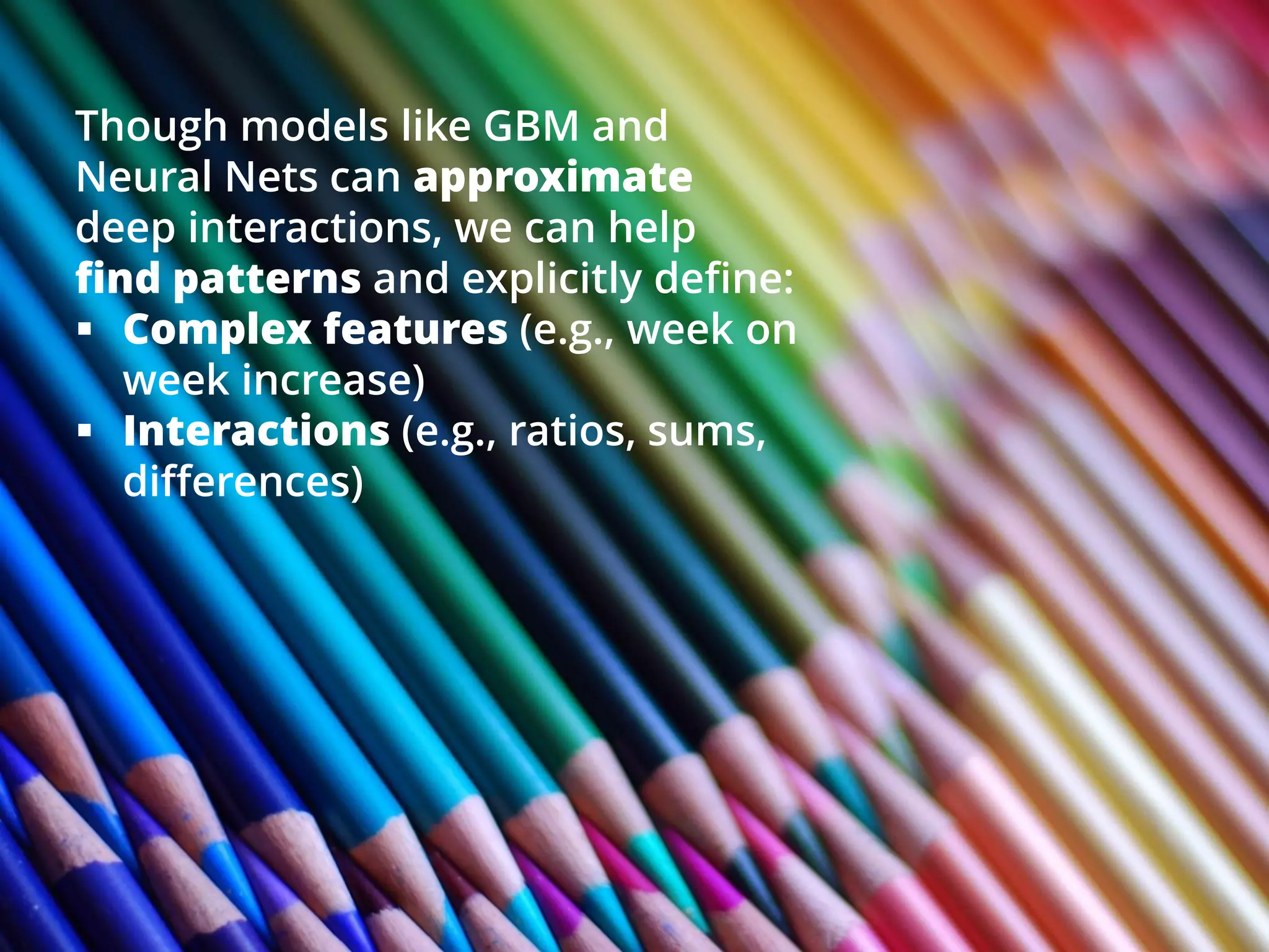
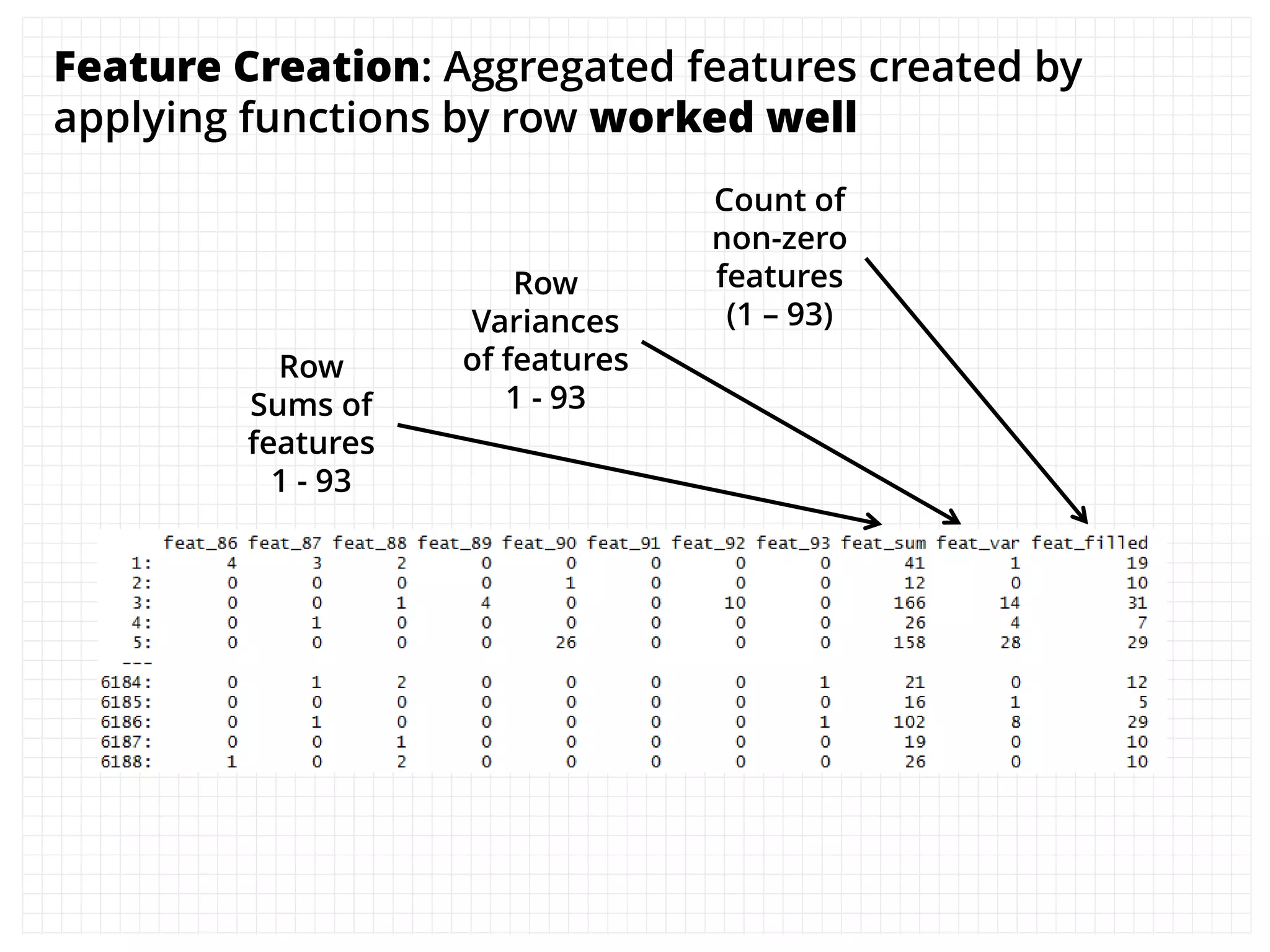
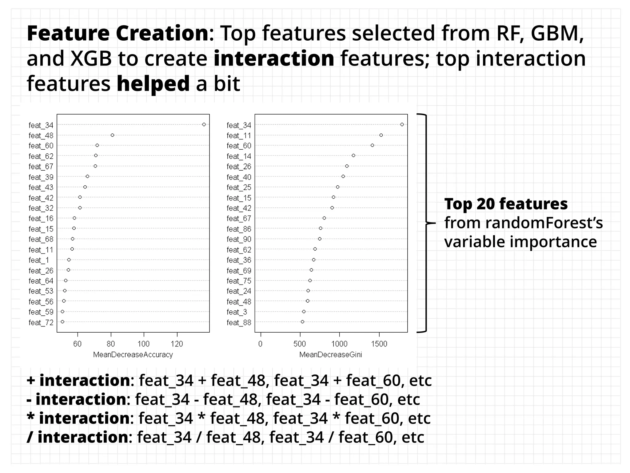
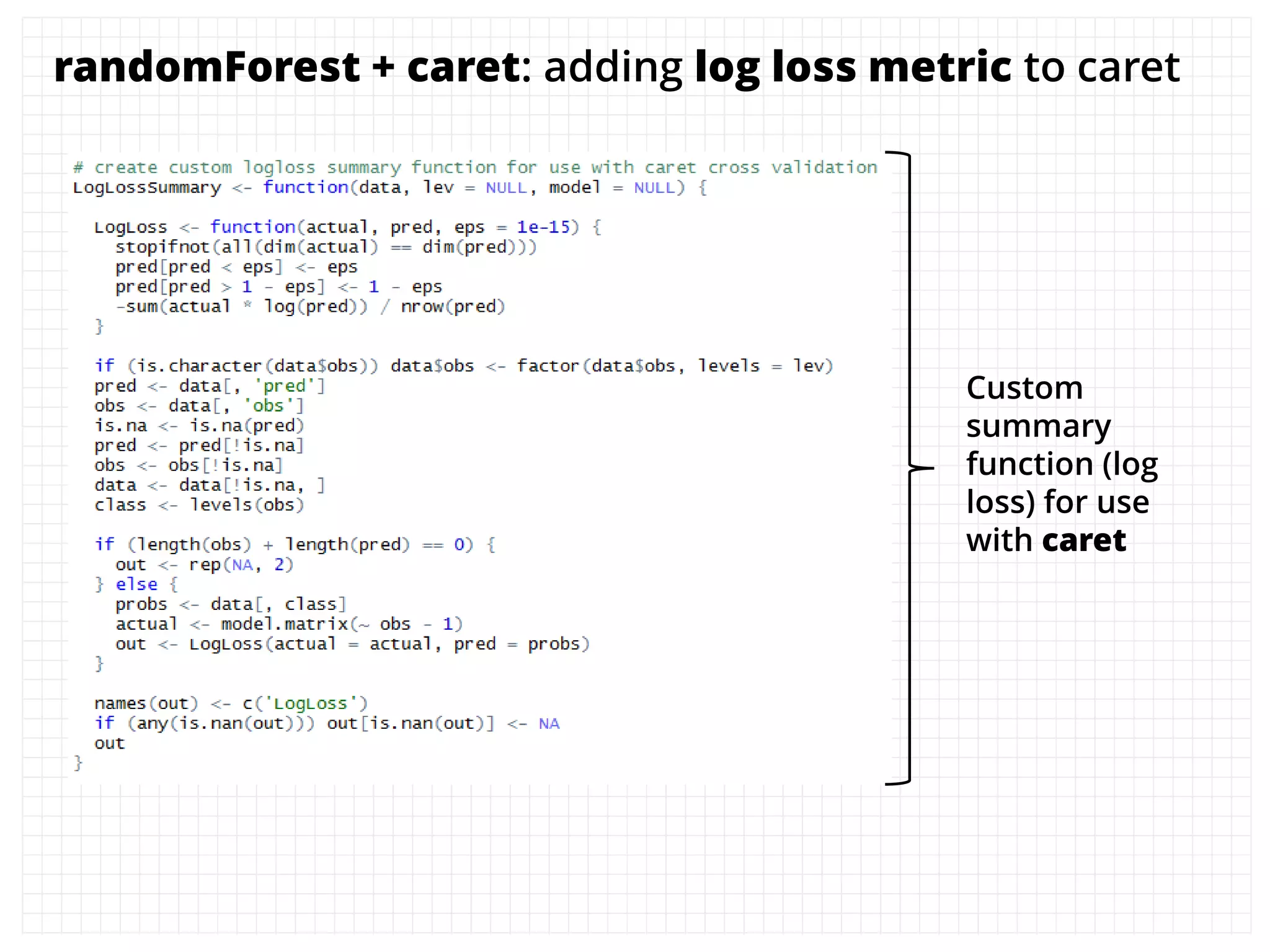
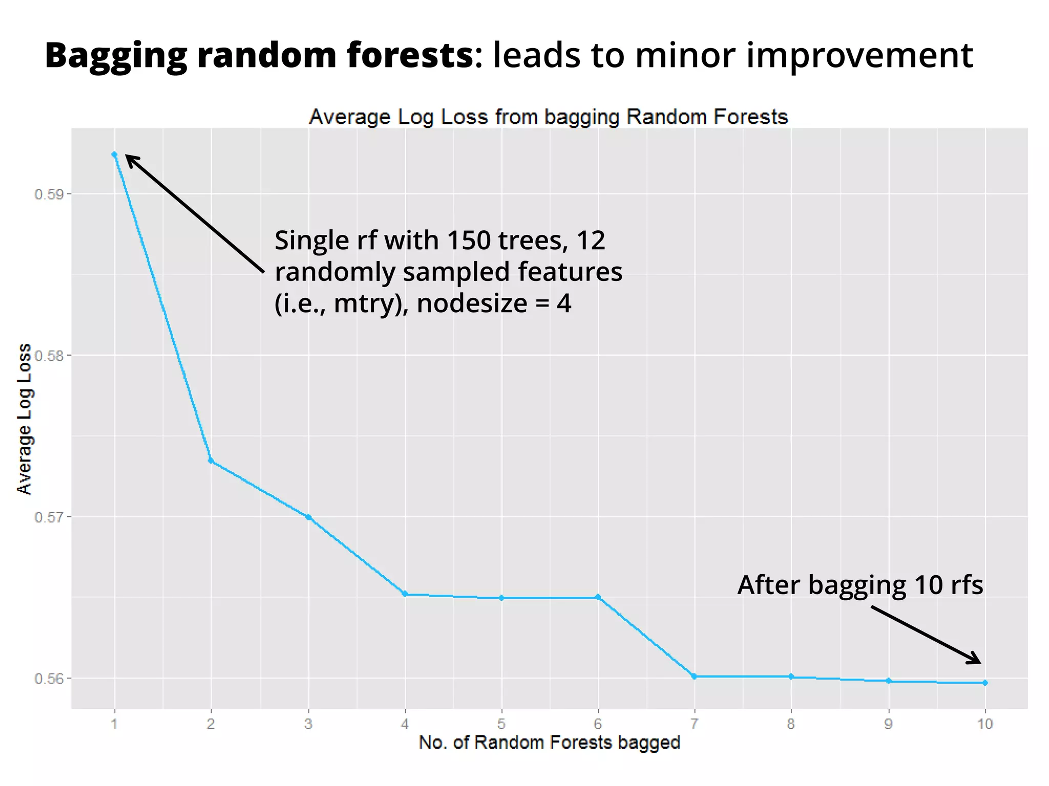
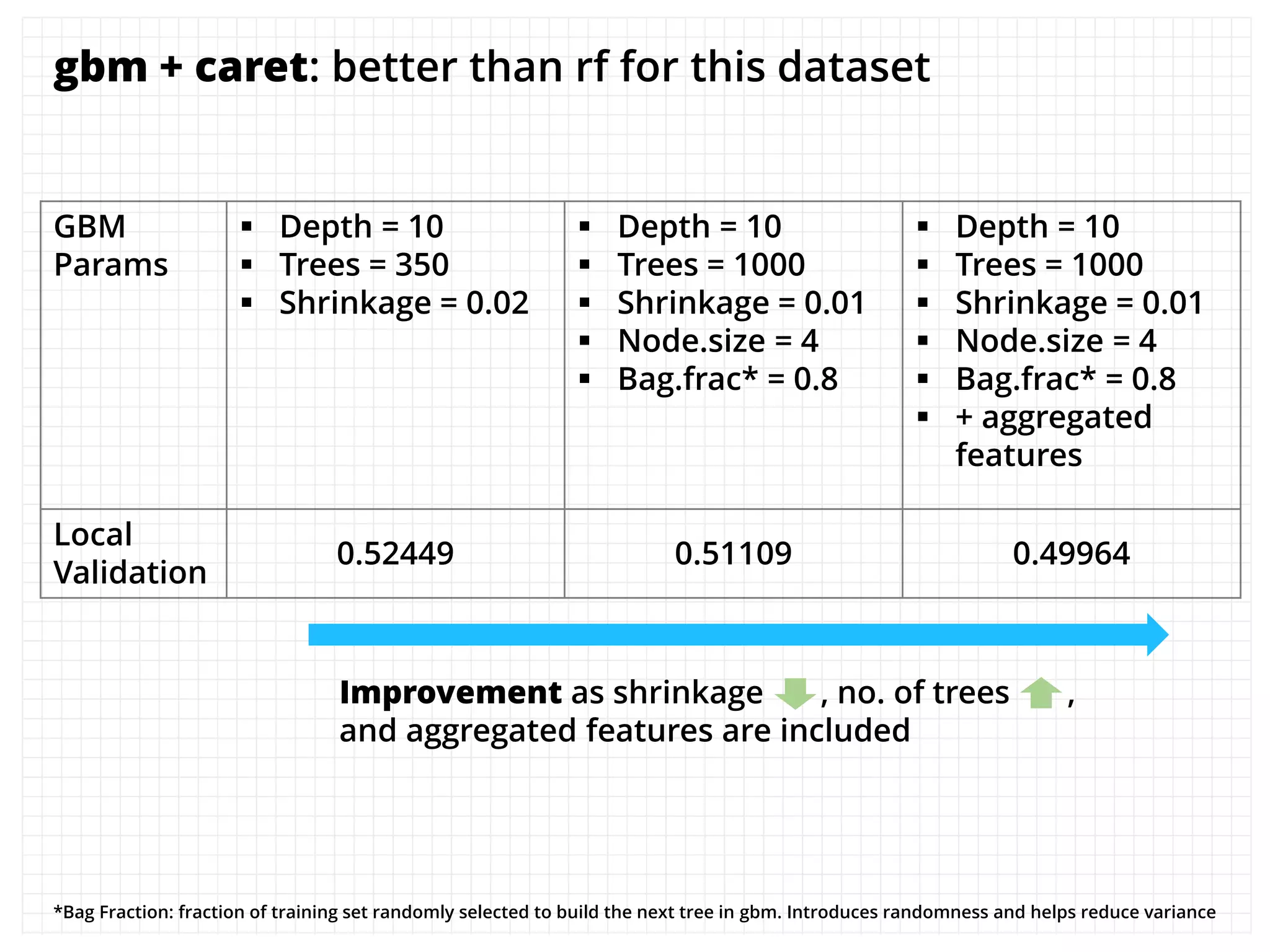
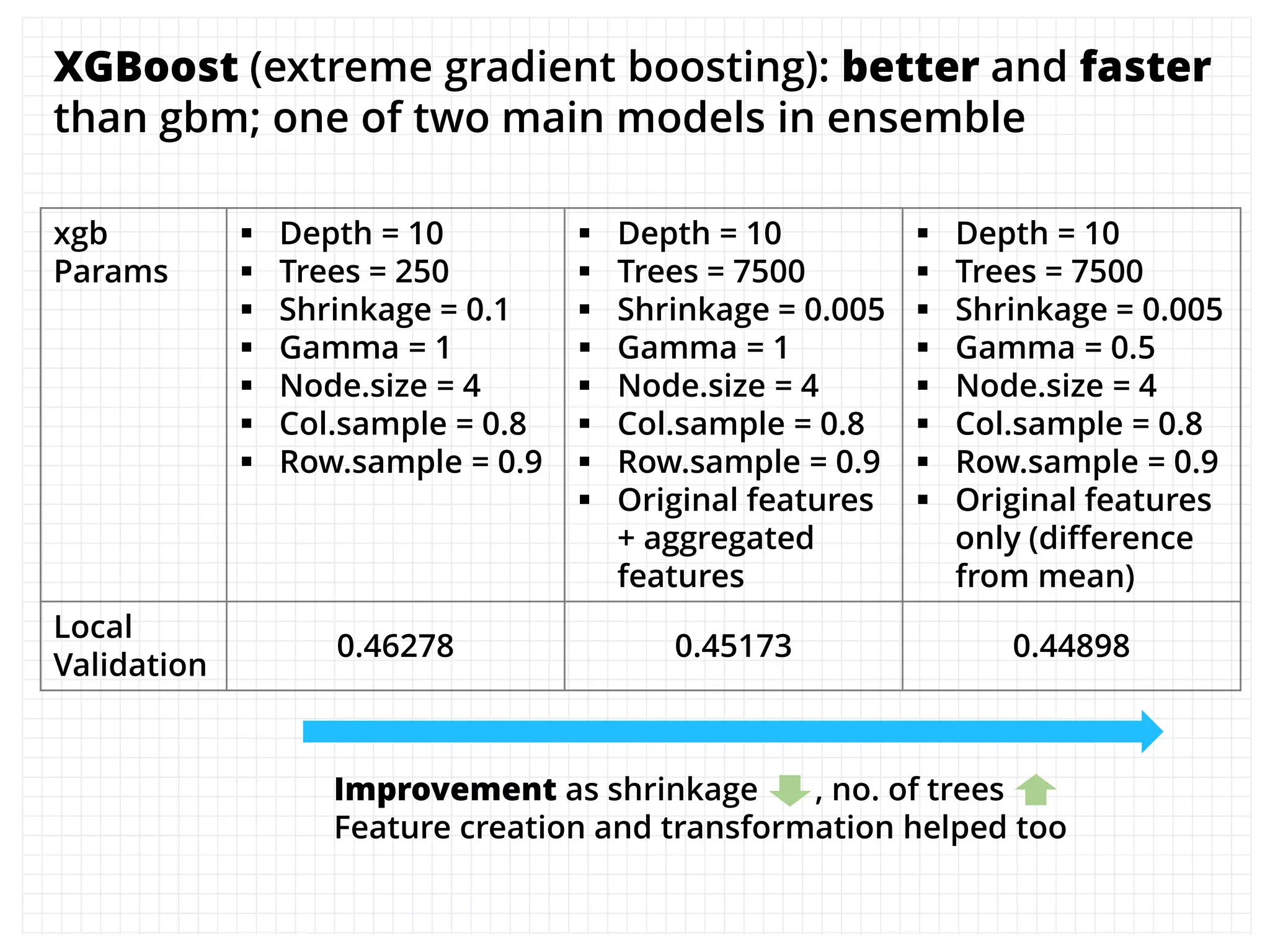
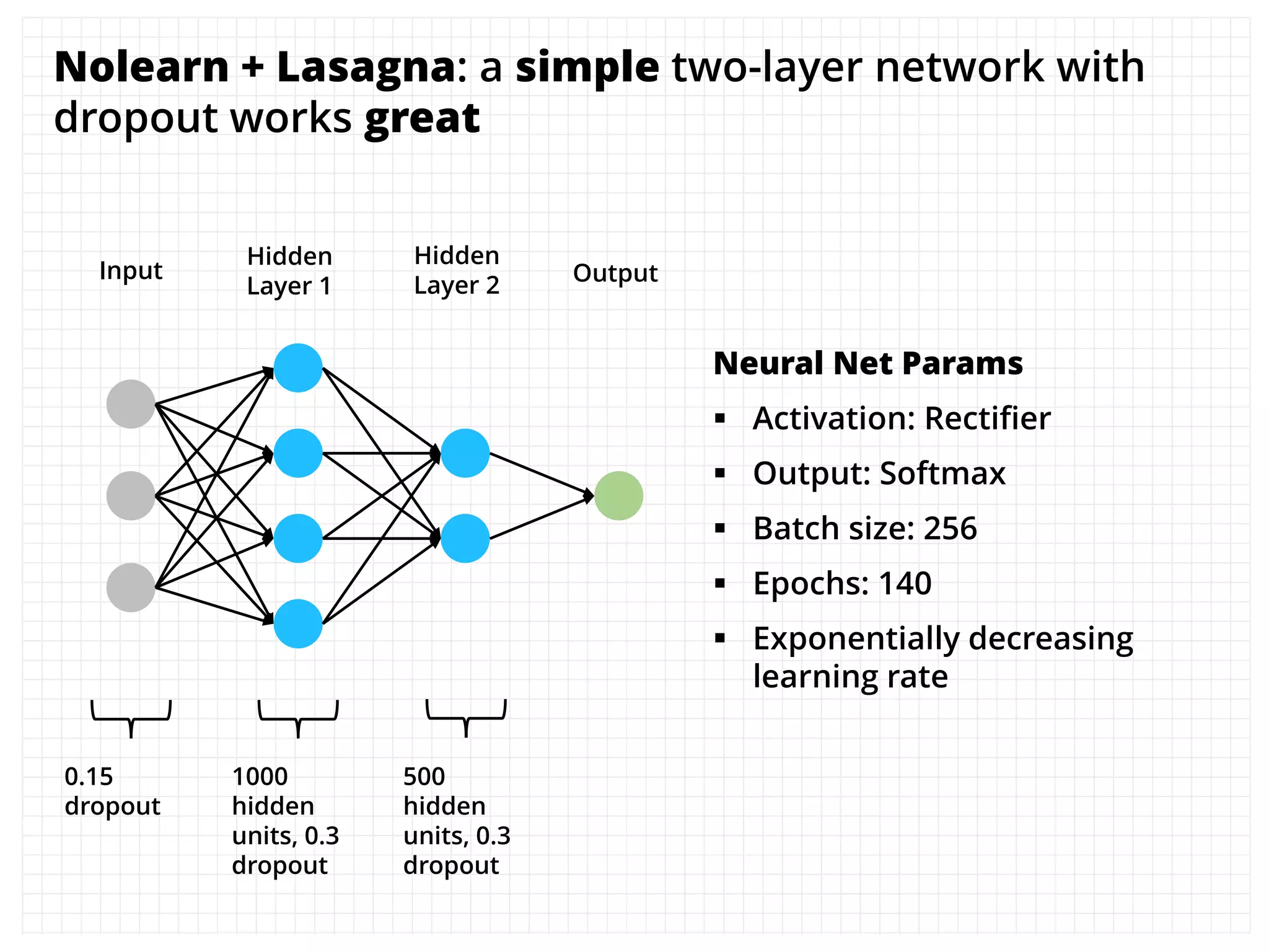
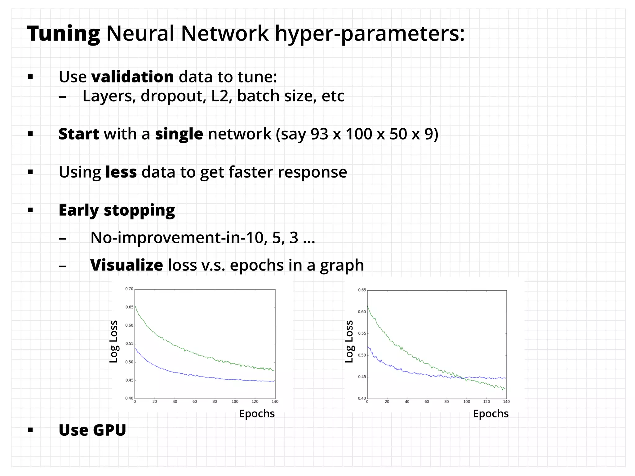
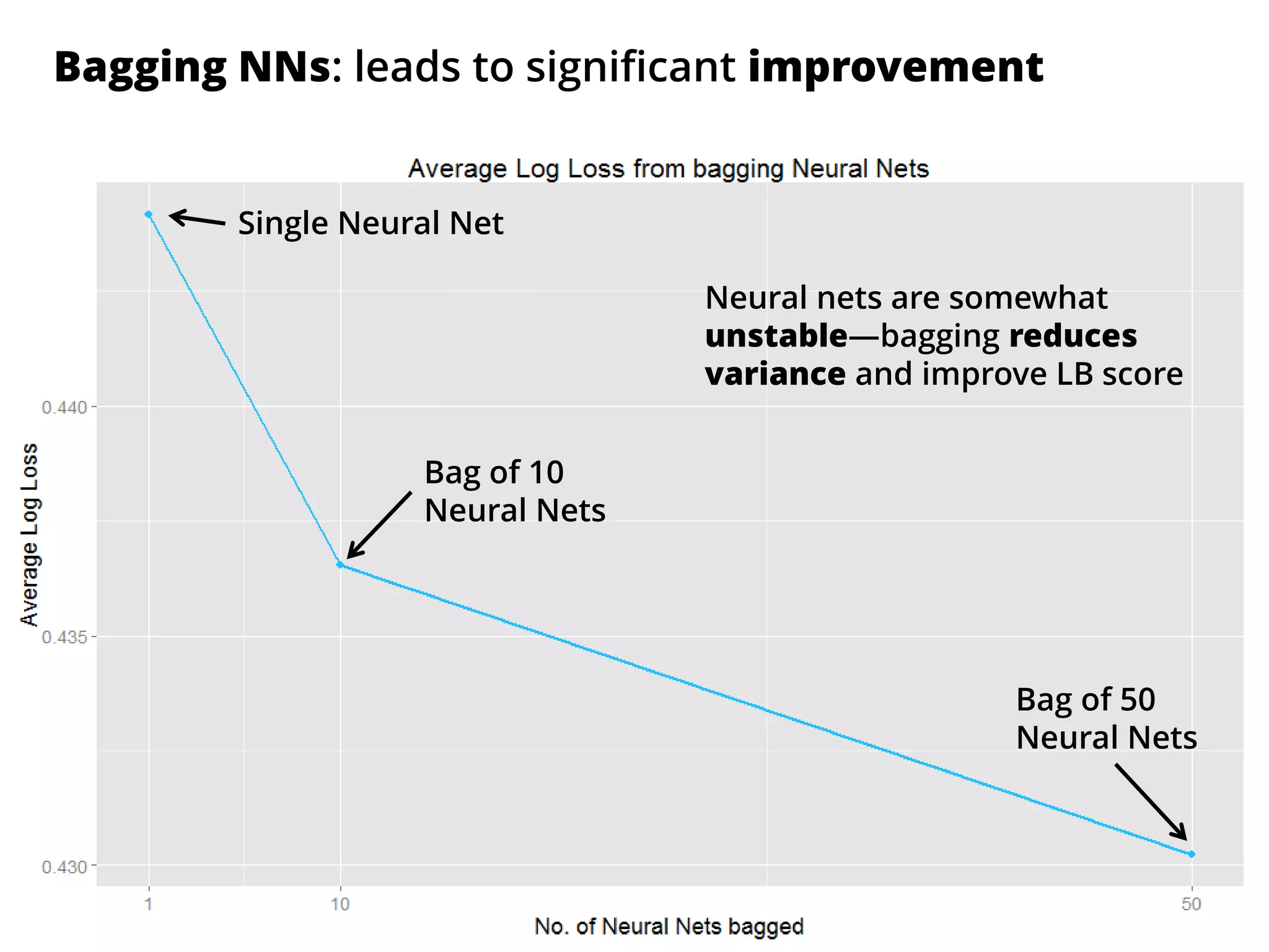
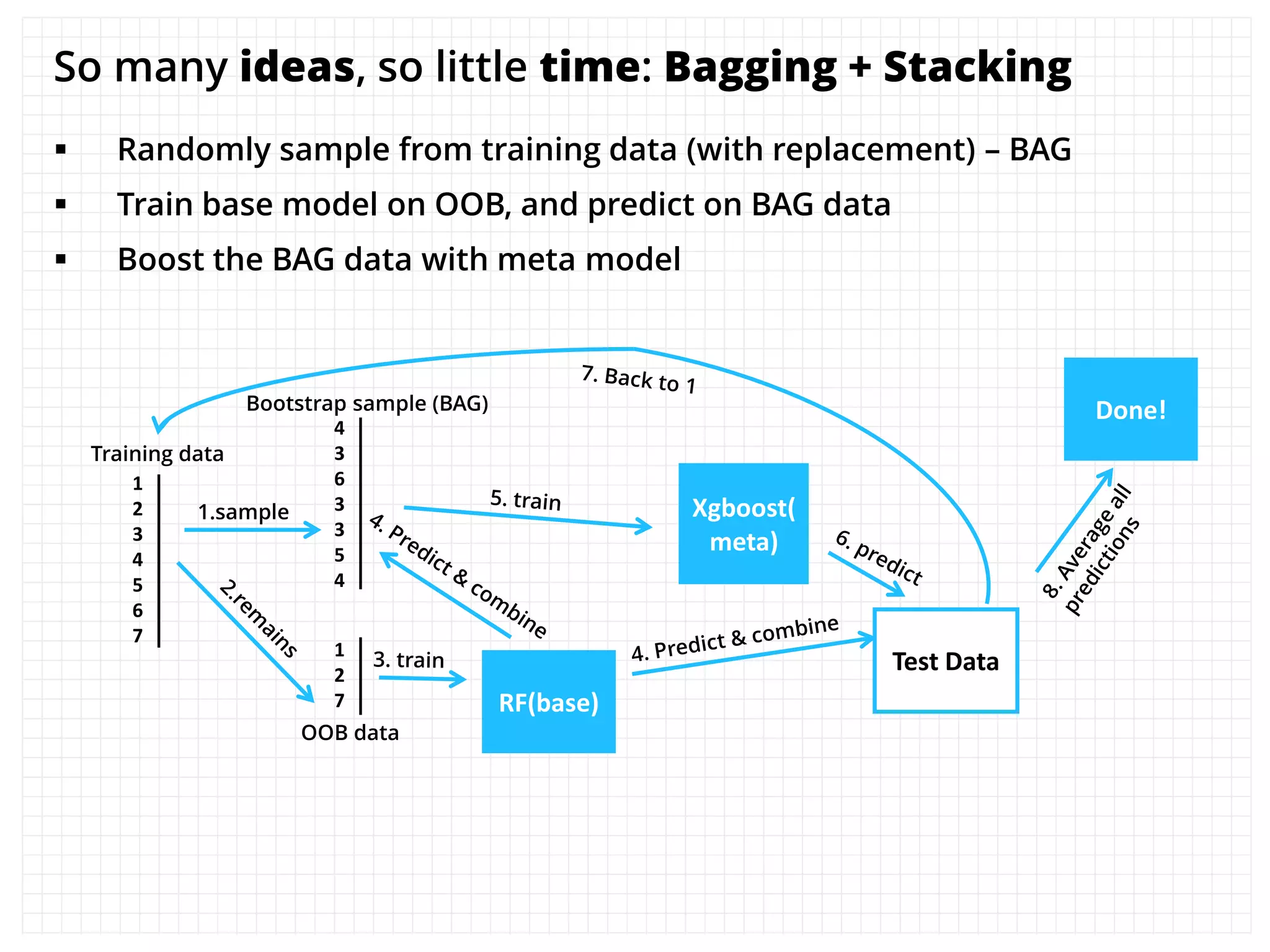
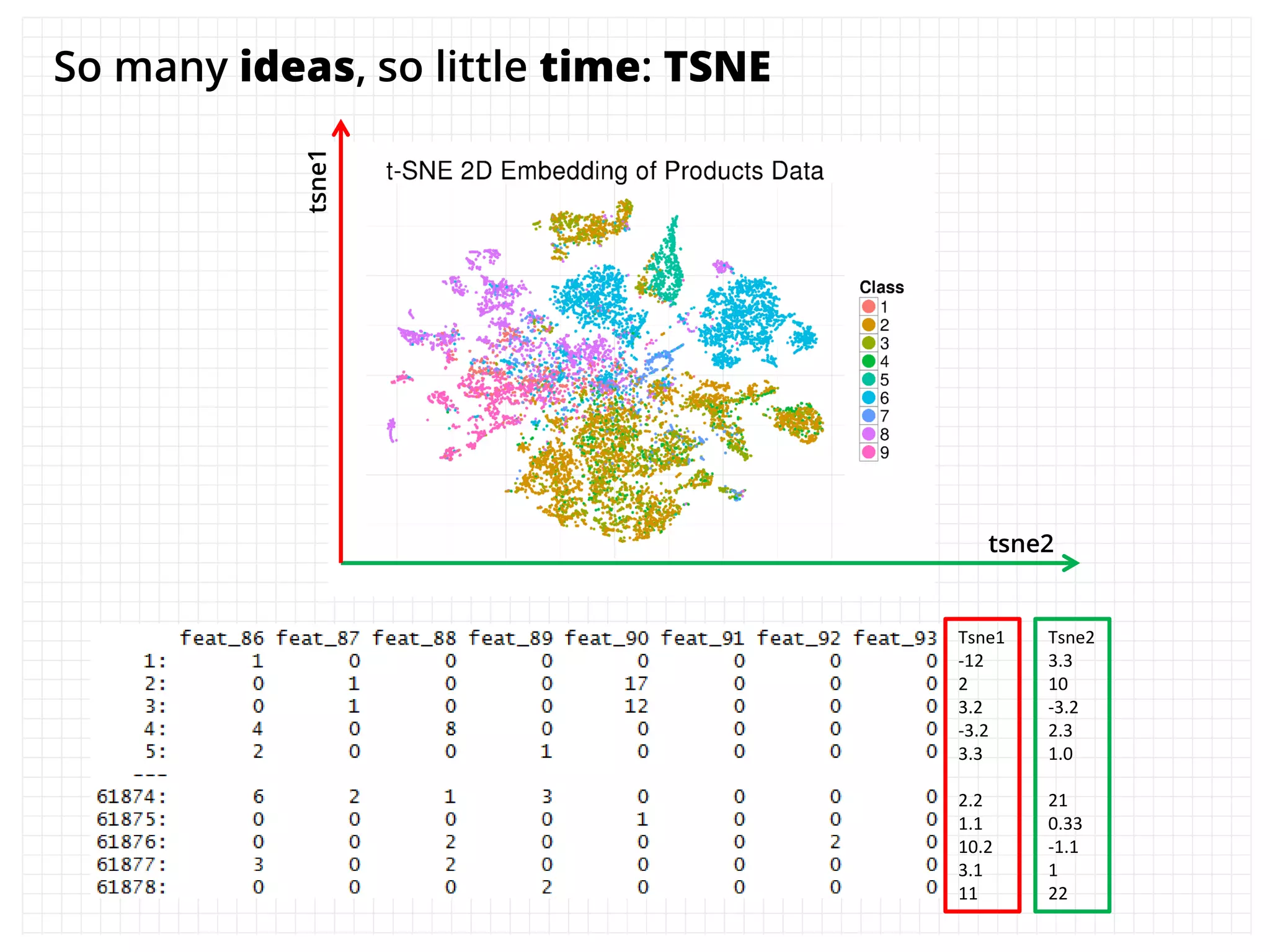
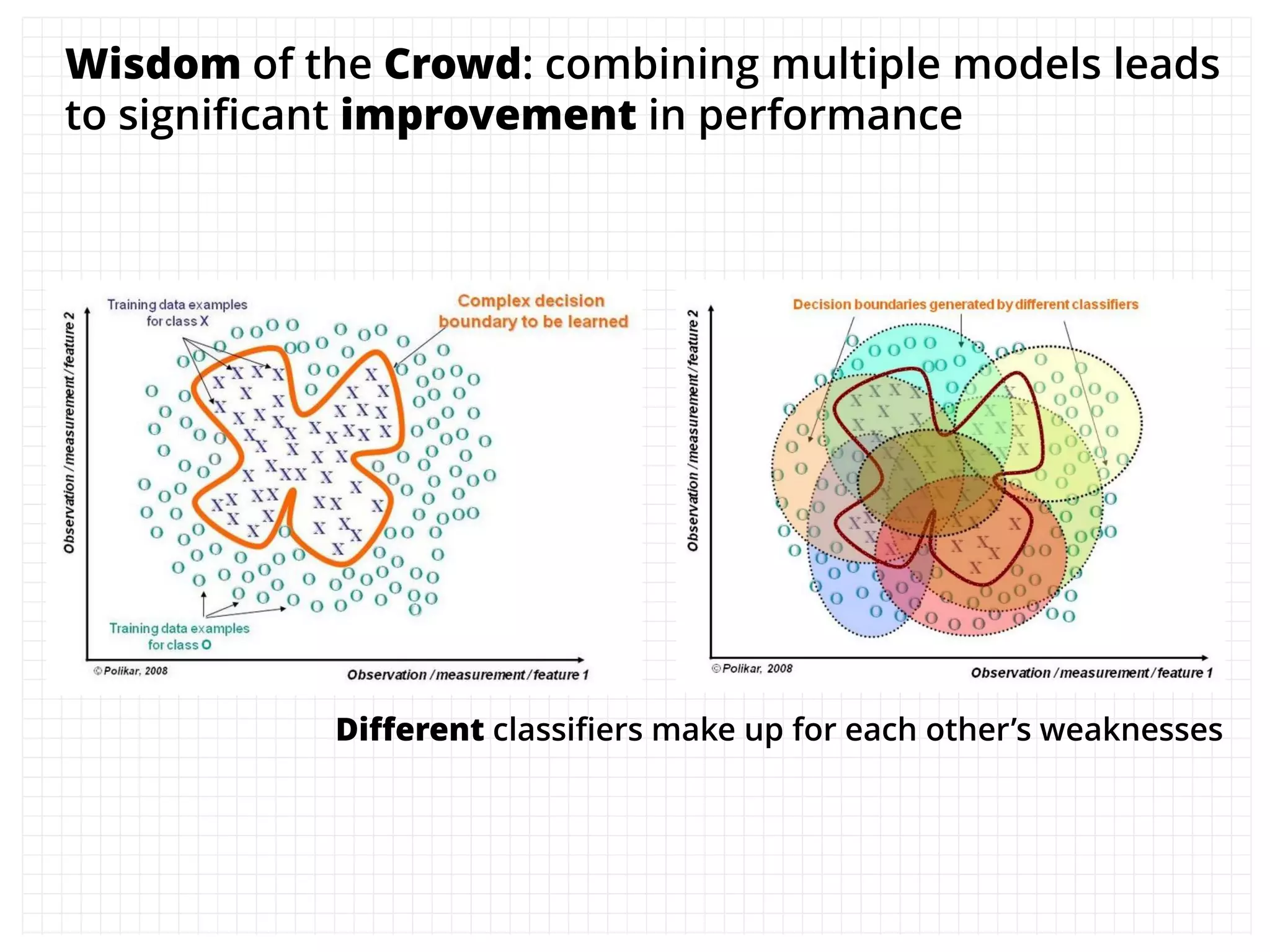
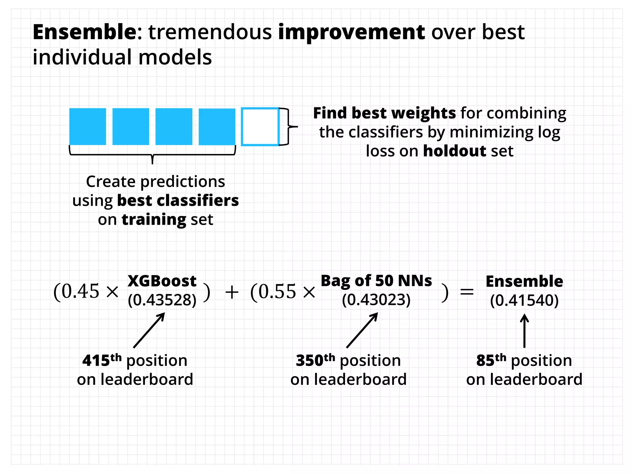
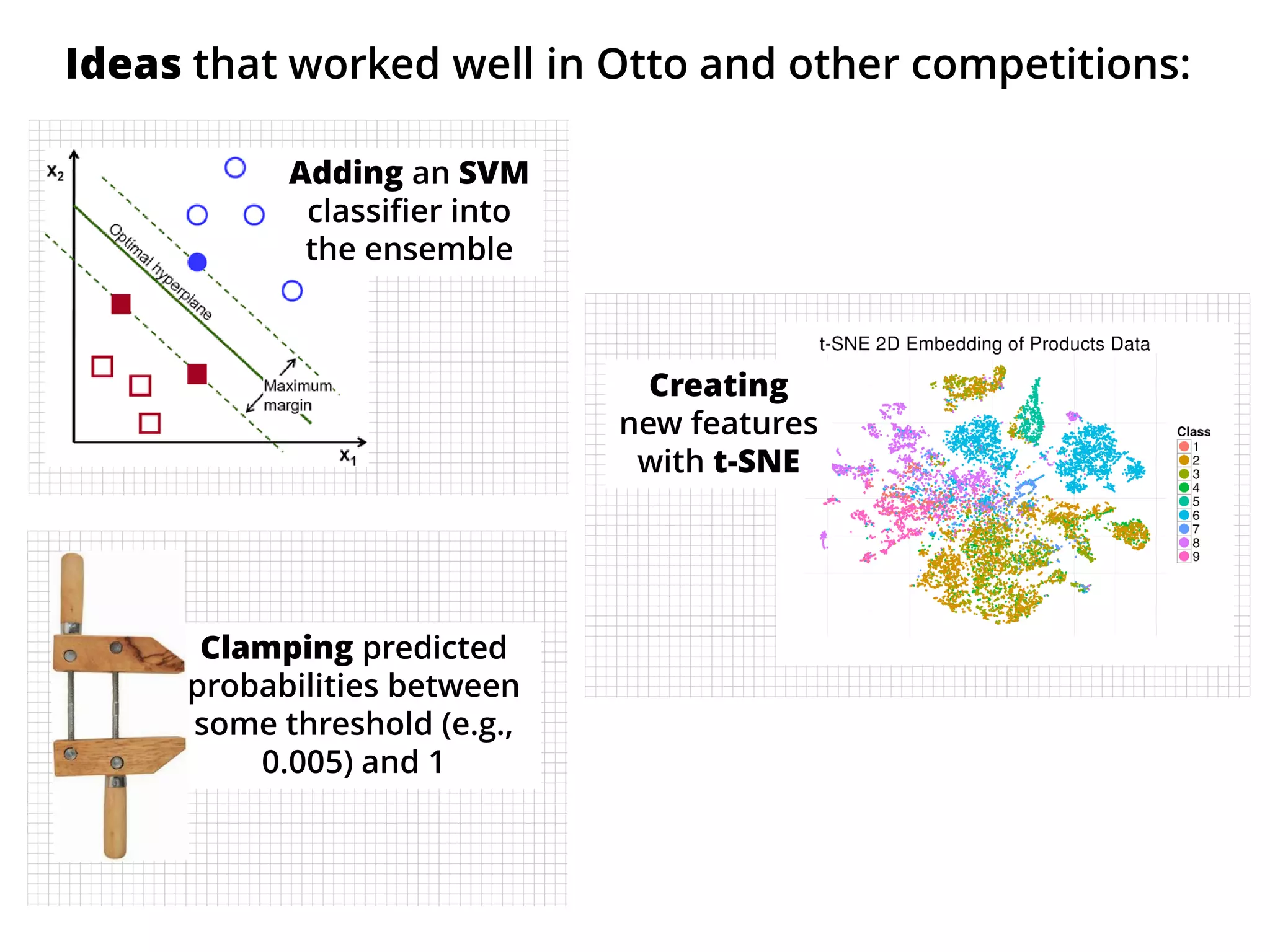
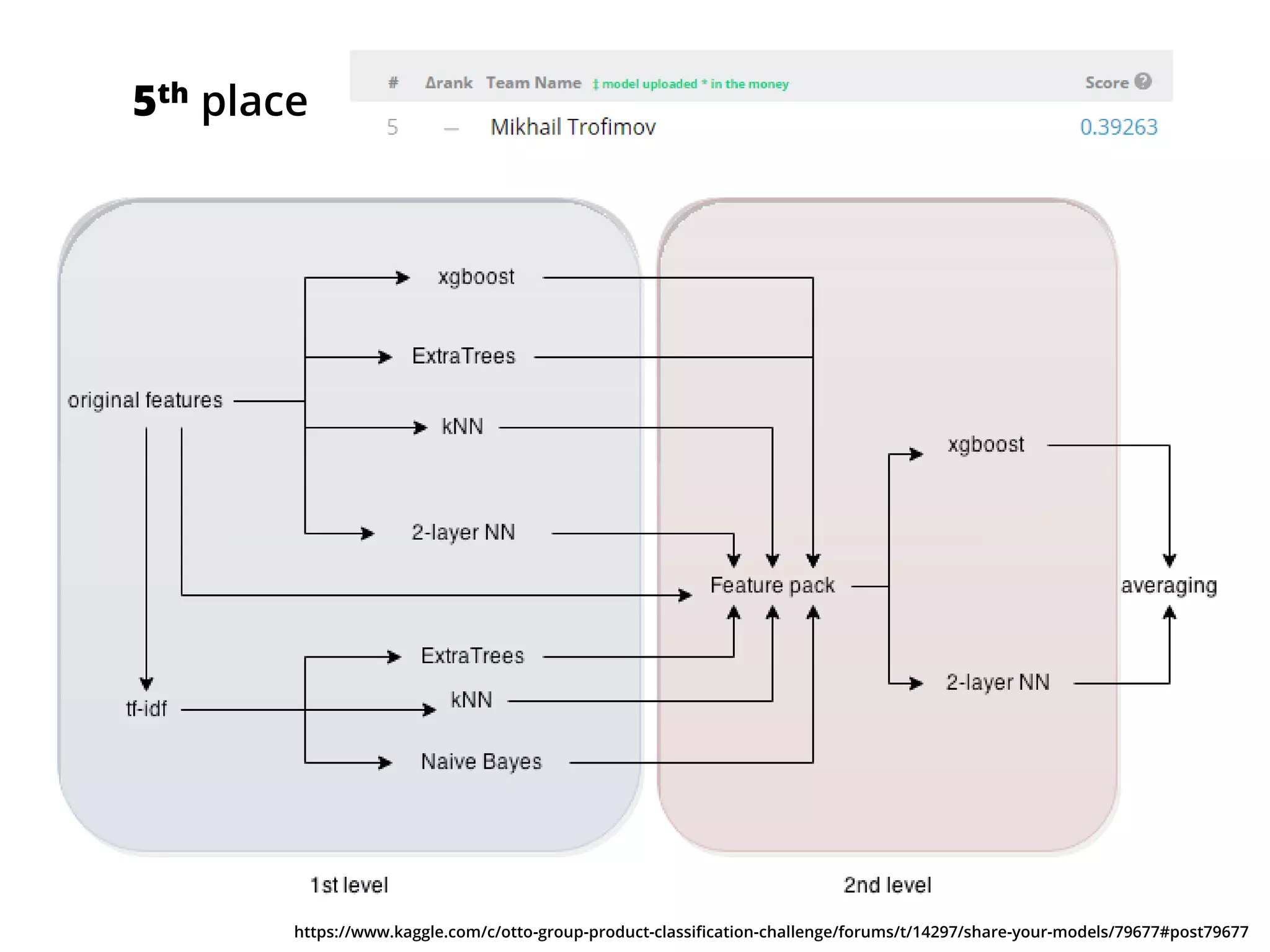
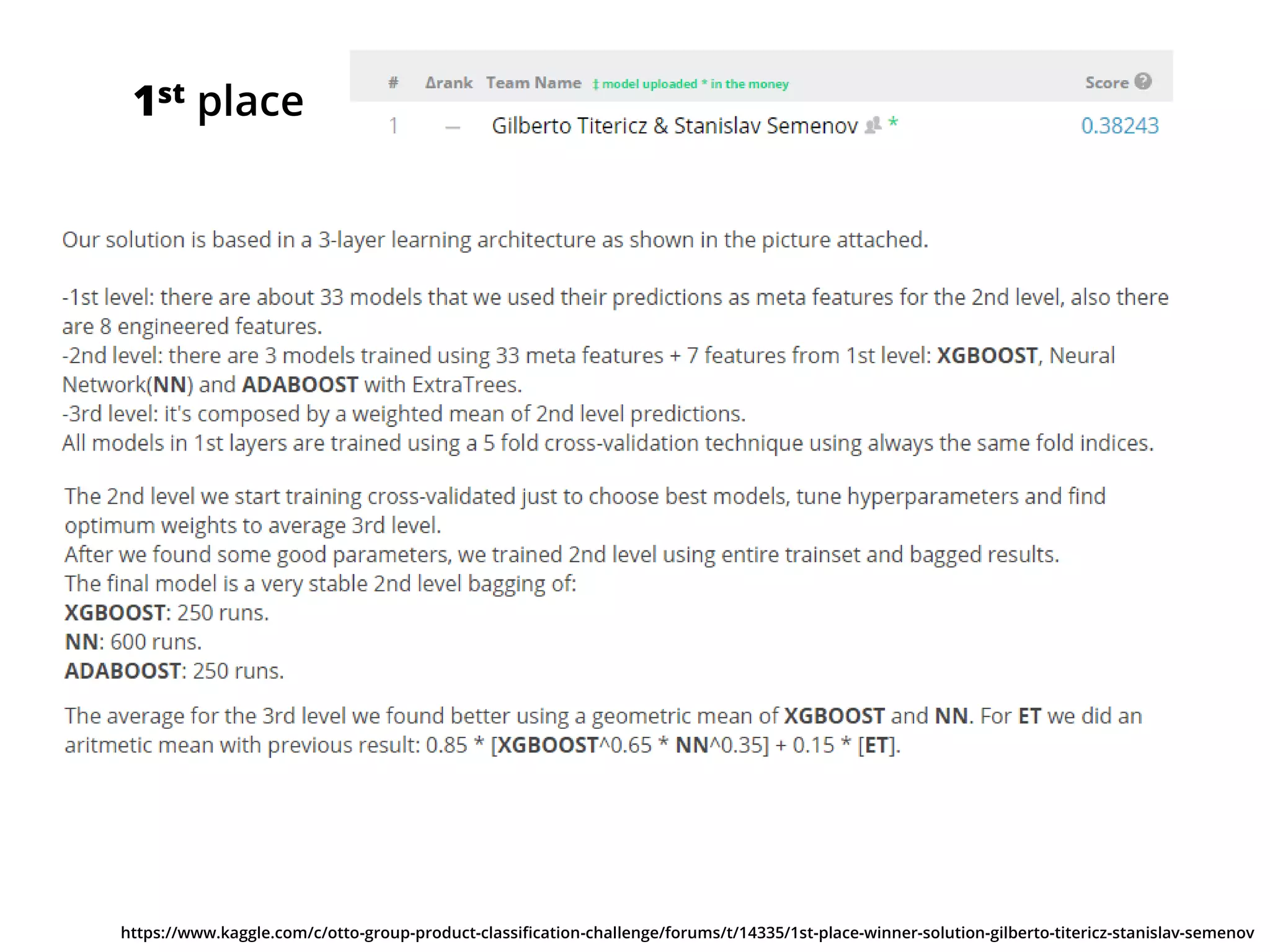
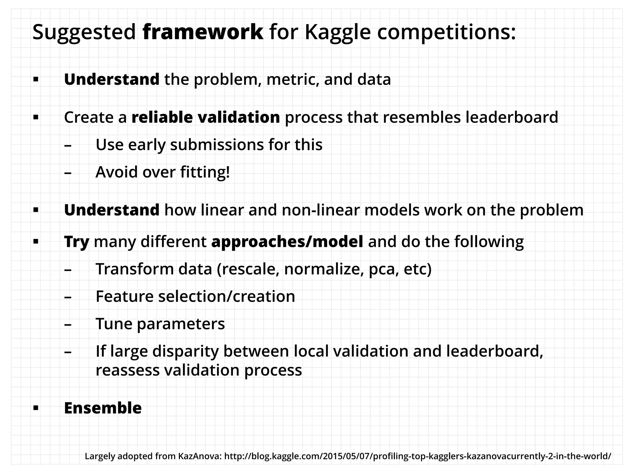
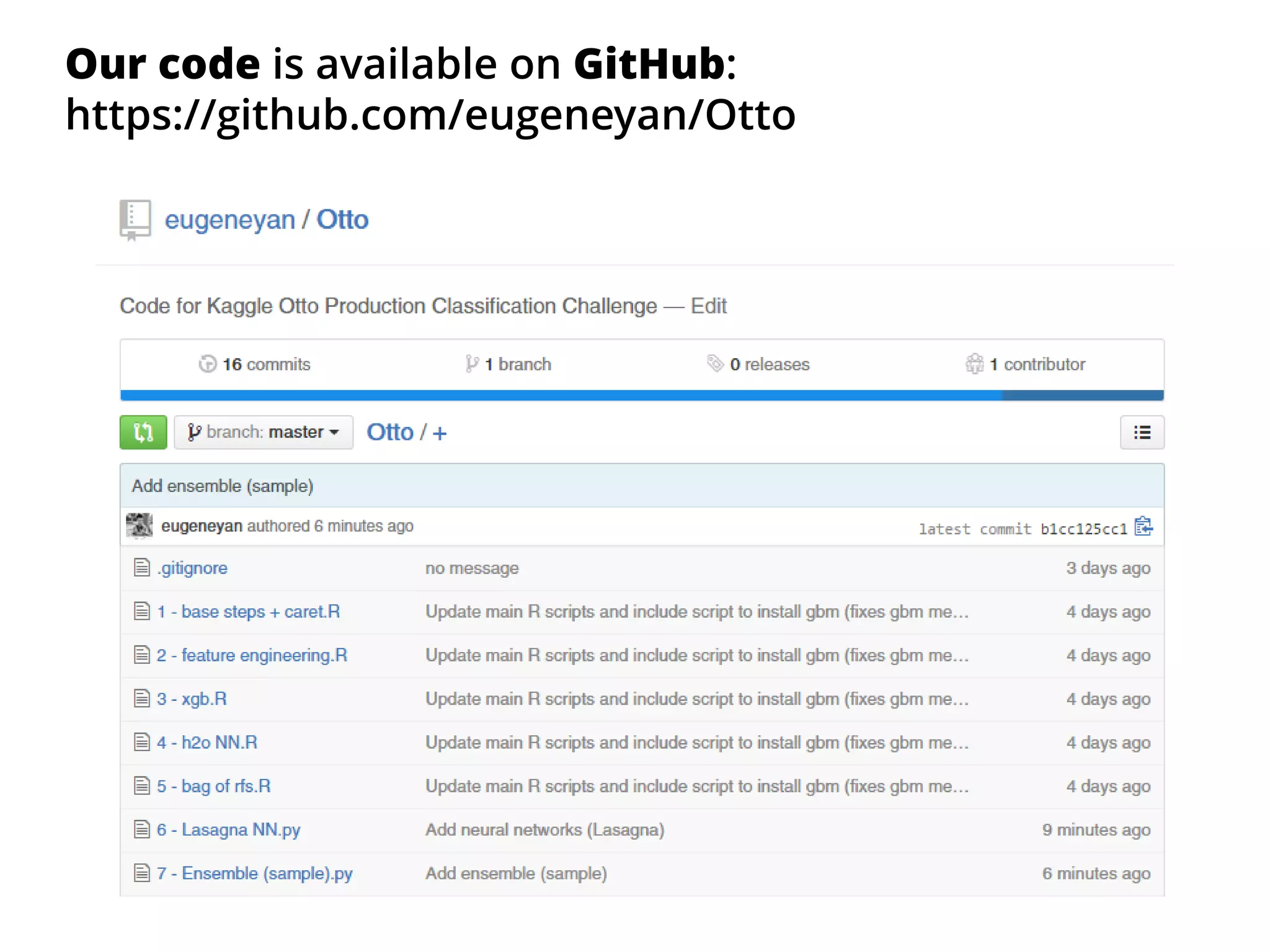
The document outlines how the authors achieved the 85th position out of 3,514 teams in the Kaggle Otto product classification challenge, focused on minimizing multi-class log loss through various modeling techniques. They discuss data feature engineering, model validation methods, and the performance of different algorithms, including tree-based models and neural networks, while emphasizing the importance of ensemble methods. The authors also provide insights into strategies for Kaggle competitions, including effective validation processes and feature transformation techniques.

1. Kaggle Otto Challenge
How we achieved 85th out of 3,514 and what we learnt
Eugene Yan & Wang Weimin

2. Kaggle: A platform for predictive modeling competitions

3. Otto Production Classification
Challenge: Classify products
into 9 main product
categories

4. One of the most popular Kaggle
competitions ever
… …
Our team achieved
85th position out of
3,514 teams

5. … …
93 (obfuscated) numerical
features provided
Target with 9
categories
Let’s take a look at the data

6. Evaluation Metric: (minimize) multi-class log loss
𝑁 = no. of products in dataset (
𝑀 = no. of class labels (i.e., 9 classes)
𝑙𝑜𝑔 = natural logarithm
𝑦𝑖𝑗 = 1 if observation 𝑖 is in class 𝑗 and 0 otherwise
𝑝𝑖𝑗 = predicted probability that observation 𝑖 belongs to class 𝑗
Minimizing multi-class log loss
heavily penalizes falsely
confident predictions

7. Validation (two
main approaches)

8. Training set Holdout
Parameter tuning
using 5 fold cross-
validation
Local
validation
using
holdout
 Train models on 80% train set and
validate against 20% local holdout
 Ensemble by fitting predictions from
80% train set on 20% local holdout
 Reduces risk of overfitting leaderboard
 Build model twice for submission
– Once for local validation
– Once for leaderboard submission
Parameter tuning and
validation using 5 fold
cross-validation
 Train models on full data set with 5-
fold cross-validation
 Build model once for submission
 Low risk of overfitting if cv score is
close to leaderboard score (i.e., training
data similar to testing data)

9. Feature
Engineering

10. Do we need all 93 features?
Can we reduce noise to
reveal more of the signal?

11. Dimensionality reduction
led nowhere: No clear ‘elbow’
from principal components
analysis

12. L1 regularization (lasso) L2 regularization
Feature Selection via elastic net/lasso dropped four
features, but led to significant drop in accuracy

13. The data looks is very skewed—
should we make it more ‘normal’?
Would standardizing/ rescaling
the data help?

14. Feature Transformation: Surprisingly, transforming
features helped with tree-based techniques
z-standardization:
𝑥 − 𝑚𝑒𝑎𝑛(𝑥)
𝑠𝑡𝑎𝑛𝑑𝑎𝑟𝑑 𝑑𝑒𝑣𝑖𝑎𝑡𝑖𝑜𝑛 (𝑥)
Difference from Mean: 𝑥 − 𝑚𝑒𝑎𝑛 𝑥
Difference from Median: 𝑥 − 𝑚𝑒𝑑𝑖𝑎𝑛 𝑥
Log-transformation: 𝑙𝑜𝑔(𝑥 + 1)
Adding flags: 𝑖𝑓 𝑥 > 0, 𝑡ℎ𝑒𝑛 1, 𝑒𝑙𝑠𝑒 0
Improved tree-
based models a bit
Worked better than
z-standardization
Didn’t help (because
most medians were 0)
Helped with Neural
Networks
Terrible =/

15. Though models like GBM and
Neural Nets can approximate
deep interactions, we can help
find patterns and explicitly define:
 Complex features (e.g., week on
week increase)
 Interactions (e.g., ratios, sums,
differences)

16. Feature Creation: Aggregated features created by
applying functions by row worked well
Row
Sums of
features
1 - 93
Row
Variances
of features
1 - 93
Count of
non-zero
features
(1 – 93)

17. Feature Creation: Top features selected from RF, GBM,
and XGB to create interaction features; top interaction
features helped a bit
+ interaction: feat_34 + feat_48, feat_34 + feat_60, etc
- interaction: feat_34 - feat_48, feat_34 - feat_60, etc
* interaction: feat_34 * feat_48, feat_34 * feat_60, etc
/ interaction: feat_34 / feat_48, feat_34 / feat_60, etc
Top 20 features
from randomForest’s
variable importance

18. Tree-based Models

19. R’s caret: adding custom log loss metric
Custom
summary
function (log
loss) for use
with caret

20. Bagging random forests: leads to minor improvement
Single rf with 150 trees, 12
randomly sampled features
(i.e., mtry), nodesize = 4
After bagging 10 rfs

21. gbm + caret: better than rf for this dataset
GBM
Params
 Depth = 10
 Trees = 350
 Shrinkage = 0.02
 Depth = 10
 Trees = 1000
 Shrinkage = 0.01
 Node.size = 4
 Bag.frac* = 0.8
 Depth = 10
 Trees = 1000
 Shrinkage = 0.01
 Node.size = 4
 Bag.frac* = 0.8
 + aggregated
features
Local
Validation
0.52449 0.51109 0.49964
Improvement as shrinkage , no. of trees ,
and aggregated features are included
*Bag Fraction: fraction of training set randomly selected to build the next tree in gbm. Introduces randomness and helps reduce variance

22. XGBoost (extreme gradient boosting): better and faster
than gbm; one of two main models in ensemble
xgb
Params
 Depth = 10
 Trees = 250
 Shrinkage = 0.1
 Gamma = 1
 Node.size = 4
 Col.sample = 0.8
 Row.sample = 0.9
 Depth = 10
 Trees = 7500
 Shrinkage = 0.005
 Gamma = 1
 Node.size = 4
 Col.sample = 0.8
 Row.sample = 0.9
 Original features
+ aggregated
features
 Depth = 10
 Trees = 7500
 Shrinkage = 0.005
 Gamma = 0.5
 Node.size = 4
 Col.sample = 0.8
 Row.sample = 0.9
 Original features
only (difference
from mean)
Local
Validation
0.46278 0.45173 0.44898
Improvement as shrinkage , no. of trees
Feature creation and transformation helped too

23. Neural Networks

24. Nolearn + Lasagna: a simple two-layer network with
dropout works great
0.15
dropout
1000
hidden
units, 0.3
dropout
500
hidden
units, 0.3
dropout
Neural Net Params
 Activation: Rectifier
 Output: Softmax
 Batch size: 256
 Epochs: 140
 Exponentially decreasing
learning rate
Input
Hidden
Layer 1
Hidden
Layer 2 Output

25. Tuning Neural Network hyper-parameters:
 Use validation data to tune:
– Layers, dropout, L2, batch size, etc
 Start with a single network (say 93 x 100 x 50 x 9)
 Using less data to get faster response
 Early stopping
– No-improvement-in-10, 5, 3 …
– Visualize loss v.s. epochs in a graph
 Use GPU
LogLoss
Epochs
LogLoss
Epochs

26. Bagging NNs: leads to significant improvement
Single Neural Net
Bag of 10
Neural Nets
Bag of 50
Neural Nets
Neural nets are somewhat
unstable—bagging reduces
variance and improve LB score

27. So many ideas, so little time: Bagging + Stacking
 Randomly sample from training data (with replacement) – BAG
 Train base model on OOB, and predict on BAG data
 Boost the BAG data with meta model
1
2
3
4
5
6
7
Training data
4
3
6
3
3
5
4
1
2
7
Bootstrap sample (BAG)
OOB data
1.sample Xgboost(
meta)
RF(base)
Test Data
Done!

28. So many ideas, so little time: TSNE
tsne1
tsne2
Tsne1
-12
2
3.2
-3.2
3.3
2.2
1.1
10.2
3.1
11
Tsne2
3.3
10
-3.2
2.3
1.0
21
0.33
-1.1
1
22

29. Ensemble our models

30. Wisdom of the Crowd: combining multiple models leads
to significant improvement in performance
Different classifiers make up for each other’s weaknesses

31. Ensemble: how do we combine to minimize log loss
over multiple models?
Create predictions
using best classifiers
on training set
 Find best weights for combining
the classifiers by minimizing log
loss on holdout set
 Our approach:
– Append various predictions
– Minimize overall log loss using
scipy.optimize.minimize
 Competition Metric: the
goal is to minimize log loss
– How to do this over
multiple models?
– Voting? Averaging?

32. Ensemble: great improvement over best individual
models, though we shouldn’t throw in everything
XGBoost
(0.43528)
Bag of 50 NNs
(0.43023)
Ensemble
(0.41540)
(0.45 × ) + (0.55 × ) =
415th position
on leaderboard
350th position
on leaderboard
85th position
on leaderboard
Our final ensemble
0.445 × XGBoost
0.545 × =Bag of 110 NNs
0.01 × Bag of 10 RFs
Ensemble
(0.41542)
+
+
Another ensemble we tried:
Sometimes, more ≠ better!

33. Ideas we didn’t have
time to implement

34. Ideas that worked well in Otto and other competitions:
Clamping predicted
probabilities between
some threshold (e.g.,
0.005) and 1
Adding an SVM
classifier into
the ensemble
Creating
new features
with t-SNE

35. Top Solutions

36. 5th place
https://www.kaggle.com/c/otto-group-product-classification-challenge/forums/t/14297/share-your-models/79677#post79677
 Use TF-IDF to transform raw features
 Create new features by fitting models on raw and TF-IDF features
 Combine created features with original features
 Bag XGBoost and 2-layer NN 30 times and average predictions

37. 2nd place
http://blog.kaggle.com/2015/06/09/otto-product-classification-winners-interview-2nd-place-alexander-guschin/
 Level 0: Split the data into two groups, Raw and TF-IDF
 Level 1: Create metafeature using different models
– Split data into k folds, training k models on k-1 parts and predict
on the 1 part left aside for each k-1 group
 Level 2: Train metaclassifier with features and metafeatures and
average/ensemble

38. 1st place
https://www.kaggle.com/c/otto-group-product-classification-challenge/forums/t/14335/1st-place-winner-solution-gilberto-titericz-stanislav-semenov

39. What’s a suggested
framework for
Kaggle?

40. Suggested framework for Kaggle competitions:
 Understand the problem, metric, and data
 Create a reliable validation process that resembles leaderboard
– Use early submissions for this
– Avoid over fitting!
 Understand how linear and non-linear models work on the problem
 Try many different approaches/model and do the following
– Transform data (rescale, normalize, pca, etc)
– Feature selection/creation
– Tune parameters
– If large disparity between local validation and leaderboard,
reassess validation process
 Ensemble
Largely adopted from KazAnova: http://blog.kaggle.com/2015/05/07/profiling-top-kagglers-kazanovacurrently-2-in-the-world/

41. Our code is available on GitHub:
https://github.com/eugeneyan/Otto

42. Thank you!
Eugene Yan
eugeneyanziyou@gmail.com
Wang Weimin
wangweimin888@yahoo.com
&