The document discusses analytical and numerical solutions for parallel flow in a channel. Analytical solutions are obtained by integrating the governing boundary value problem using methods like series expansion, resulting in an approximate solution. The solution is expressed as a function of the independent variables in a series form, with accuracy depending on the number of terms included. Numerical solutions involve approximating derivatives using finite differences on a grid, resulting in an equation relating the velocity at neighboring points that can be solved iteratively.

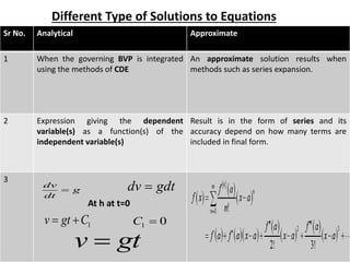
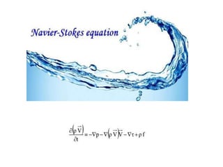
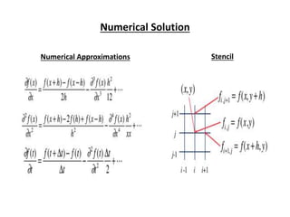
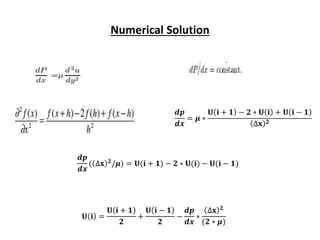
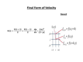
1. Navier Stokes Equation its Analytical
and Numerical Solution
Parallel Flow in Channel
Presented By: Mushahid Yasin

2. Sr No. Analytical Approximate
1 When the governing BVP is integrated
using the methods of CDE
An approximate solution results when
methods such as series expansion.
2 Expression giving the dependent
variable(s) as a function(s) of the
independent variable(s)
Result is in the form of series and its
accuracy depend on how many terms are
included in final form.
3
At h at t=0
Different Type of Solutions to Equations
dv
g
dt
 dv gdt

1
v gt C
  1 0
C 
v gt


4. Assumptions
Laminar. Steady
Incompressible 2-Dimensional

5. Parallel Flow in Channel
• Parallel flows, since the flow is constrained by the flat
parallel walls of the channel, no component of the
velocity in the y direction is possible, i.e., v= 0. This
implies
Parallel flow through a straight channel.

6. Parallel Flow in a Channel

7. Applying Assumptions
How on earth
this had
happened??
U≠f(x)
No Slip Condition

8. Final Form of Velocity
Maximum Velocity
y=0

9. Numerical Solution
Numerical Approximations Stencil

10. Numerical Solution
𝒅𝒑
𝒅𝒙
= 𝝁 ∗
𝐔 𝐢 + 𝟏 − 𝟐 ∗ 𝐔 𝐢 + 𝐔 𝐢 − 𝟏
∆𝐱 𝟐
𝒅𝒑
𝒅𝒙
( ∆𝐱 𝟐
/𝝁) = 𝐔(𝐢 + 𝟏) − 𝟐 ∗ 𝐔(𝐢) − 𝐔(𝐢 − 𝟏)
𝐔 𝐢 =
𝐔 𝐢 + 𝟏
𝟐
+
𝐔 𝐢 − 𝟏
𝟐
−
𝒅𝒑
𝒅𝒙
∗
∆𝐱 𝟐
(𝟐 ∗ 𝝁)

11. Final Form of Velocity
Stencil
𝐔 𝐢 =
𝐔 𝐢 + 𝟏
𝟐
+
𝐔 𝐢 − 𝟏
𝟐
−
𝒅𝒑
𝒅𝒙
∗
∆𝐱 𝟐
(𝟐 ∗ 𝝁)