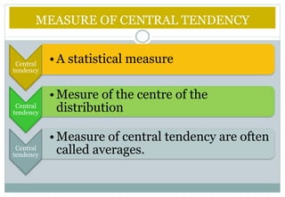
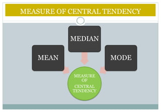
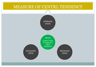
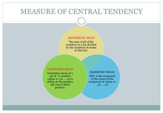
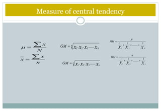
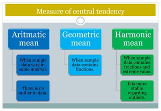
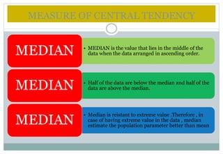
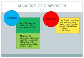
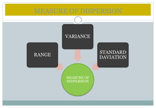
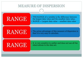
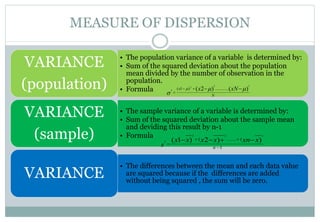
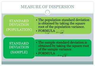
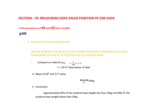
This document defines and explains various measures of central tendency and dispersion. It discusses the mean, median, mode, range, variance, and standard deviation as measures of central tendency and dispersion. It also provides the formulas to calculate the arithmetic mean, harmonic mean, geometric mean, variance, and standard deviation. Additionally, it demonstrates how to identify outliers in a data set using the lower and upper fences.

1. MEASURE OF CENTRAL
TENDENCY

2. MEASURE OF CENTRAL TENDENCY
Central
tendency
•A statistical measure
Central
tendency
•Mesure of the centre of the
distribution
Central
tendency
•Measure of central tendency are often
called averages.

3. MEASURE OF CENTRAL TENDENCY
MEASURE
OF
CENTRAL
TENDENCY
MEAN
MEDIAN
MODE

4. MEASURE OF CENTRL TENDENCY
MEAN
(mean is the
average of a
set of
numbers)
Arithmtic
mean
Harmonic
mean
Geometric
mean

5. MEASURE OF CENTRAL TENDENCY
ARITHMETIC MEAN
The sum of all of the
numbers in a list divided
by the numbers of atoms
in that list.
HARMONIC MEAN
HM is the reciprocal
of the mean of the
reciprocal of values x1
, x2……xn
GEOMETRIC MEAN
Geometric mean of a
set of ‘n’ positive
values x1 ,x2 ,….xn is
define as the positive
nth root of their
product.

6. Measure of central tendency
XXX N
N
HM
1
........
11
21


n
nxxxxGM ........ 321

N
NxxxxGM ........ 321

n
x
x

XXX n
n
HM
1
........
11
21


N
x

7. Measure of central tendency
Aritmatic
mean
When sample
data vary in
same interval.
There is no
outlier in data.
Geometric
mean
When sample
data contains
fractions.
Harmonic
mean
When sample
data contains
fractions and
extreme value.
It is more
stable
regarding
outliers.

8. MEASURE OF CENTRAL TENDENCY
• MEDIAN is the value that lies in the middle of the
data when the data arranged in ascending order.MEDIAN
• Half of the data are below the median and half of the
data are above the median.MEDIAN
• Median is reistant to extreme value .Therefore , in
case of having extreme value in the data , median
estimate the population parameter better than mean
MEDIAN

9. MEASURE OF CENTRAL TENDENCY
MODE
• MODE is the most frequent observation in the data set.
MODE
• If there are two modes , data is bimodal
• If there are three or more modes , data set is multimodal ,
typically not reported as representative of central tendency.
MODE
• Mode can be used in case of qualitative and quantitative
data.

10. MEASURE OF DISPERSION

11. MEASURE OF DISPERSION
DISPERSION also
called variability ,
scatter or spread.
Measures of
dispersion attempt to
describe the spread
of the data or its
variation around the
central value.
DIPERSION
Two distinct samples
may have the same
mean or median , but
completely different
values of
varialability.
DISPERSION

12. MEASURE OF DISPERSION
MEASURE OF
DIDPERSION
RANGE
VARIANCE
STANDARD
DAVIATION

13. MEASURE OF DISPERSION
• THE RANGE of a variable is the difference between
the largest data value and the smallest data value.
• RANGE = Largest data value – smallest data value
RANGE
• The prime advantage of this measure of dispersion is
that it is very easy to calculate.RANGE
• It is very sensitive to outlier and does not use all the
observations in the data set.
RANGE

14. MEASURE OF DISPERSION
• The population variance of a variable is determined by:
• Sum of the squared deviation about the population
mean divided by the number of observation in the
population.
• Formula
VARIANCE
(population)
• The sample variance of a variable is determined by:
• Sum of the squared deviation about the sample mean
and deviding this result by n-1
• Formula
VARIANCE
(sample)
• The differences between the mean and each data value
are squared because if the differences are added
without being squared , the sum will be zero.
VARIANCE
N
x xNx )()2(
22
2
2
.............)1( 

 

1
(.......( ))2)1(
222
2




n
xxnxxxx
s

15. MEASURE OF DISPERSION
• The population standard deviation
is obtained by taking the square
root of the population variance.
• FORMULA
STANDARD
DEVIATION
(POPULATION)
• The sample standard deviation is
obtained by taking the square root
of the sample variance.
• FORMULA
STANDARD
DEVIATION
(SAMPLE)
SS
2


2
 
2


16. SECTION – IV: MEASURING DATA VALUE POSITION IN THE DATA
1-The parameters as P40 and P82 for y-variable
p𝟒𝟎
 Arrange the data in ascending order
28,32,46,48,48,48,50,50,50,52,52,53,54,55,56,56,57,57,58,59,59,59,60,60,61,62,62,62,6
3,63,63,66,66,70,70,70,70,71,71,72,73,73,74,74,77,82,85,87,89,95
• Compute an index for 𝑝40
𝑖 = 20.4𝑡ℎ observation of data
 Mean of 20th and 21𝑡ℎ value
59+59
2
=59kg
 Conclusion
Approximately 40% of the students have weight less than 59kg and 60% of the
students have weight above than 59kg.

17. p𝟖𝟐
 Arrange the data in ascending order
28,32,46,48,48,48,50,50,50,52,52,53,54,55,56,56,57,57,58,59,59,59,60,60,61,62,62,62,63,63,63,66,66,7
0,70,70,70,71,71,72,73,73,74,74,77,82,85,87,89,95
 Compute an index for 𝑝82
𝑘
(100 ) (51+1)
82
𝑖 = (100 ) (51+1)
𝑖 = 41.82𝑡ℎ observation of data
 Mean of 41th and 42𝑡ℎ value
73+73
2
=73kg
 Conclusion
Approximately 82% of the students have weight less than 73kg and 18% of the
students have weight above than 73kg.

18. 2-outlier in the population data (y-variable)
Q1  Arrange the data in ascending order
28,32,46,48,48,48,50,50,50,52,52,53,54,55,56,56,57,57,58,59,59,59,60,60,61,62,62,62,6
3,63,63,66,66,70,70,70,70,71,71,72,73,73,74,74,77,82,85,87,89,95
 Compute an index for 𝑄1
25
𝑖 = (100 ) (50 + 1)
𝑖 = 12.75𝑡ℎ observation of data
 Mean of 12th and 13 𝑡ℎ value
53+54
2
=53.5kg
 Conclusion
Approximately 25% of the students have weight less than 53.5kg and 75% of the
students have weight above than 53.5kg.

19. 𝑸 𝟑
 Arrange the data in ascending order
28,32,46,48,48,48,50,50,50,52,52,53,54,55,56,56,57,57,58,59,59,59,60,60,61,62,62,62,6
3,63,63,66,66,70,70,70,70,71,71,72,73,73,74,74,77,82,85,87,89,95
 Compute an index for 𝑄3
75
𝑖 = (100 ) (50 + 1)𝑖 = 38.25𝑡ℎ observation of data
 Mean of 38th and 39𝑡ℎ value
71+71
2
=71kg
 Conclusion
Approximately 75% of the students have weight less than 71kg and 25% of the students
have weight above than 75kg.
IQR
𝐼𝑄𝑅 = 𝑄3-𝑄1
𝐼𝑄𝑅 = 71 − 53.
𝐼𝑄𝑅 = 17.5

20. LOWER FENCE
𝐿𝑂𝑊𝐸𝑅 𝐹𝐸𝑁𝐶𝐸 = 𝑄1 − (1.5 × 𝐼𝑄𝑅)
𝐿𝑂𝑊𝐸𝑅 𝐹𝐸𝑁𝐶𝐸 = 𝑄1 − (1.5 × 17.5)
𝐿𝑂𝑊𝐸𝑅 𝐹𝐸𝑁𝐶𝐸 = 27.25
UPPER
FENCE
𝑈𝑃𝑃𝐸𝑅 𝐹𝐸𝑁𝐶𝐸 = 𝑄3 + (1.5 × 𝐼𝑄𝑅)
𝐿𝑂𝑊𝐸𝑅 𝐹𝐸𝑁𝐶𝐸 = 71 + 27.25
𝐿𝑂𝑊𝐸𝑅 𝐹𝐸𝑁𝐶𝐸 = 98.25
Conclusion:
 No value is less than lower fence
 No value is bigger than upper fence
So there is no outlier in data.