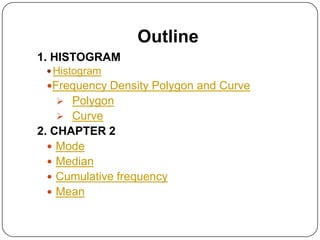
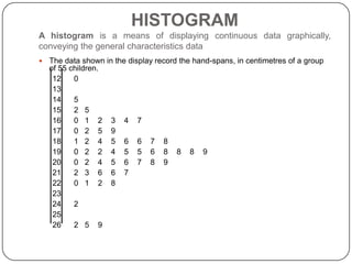
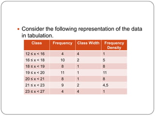
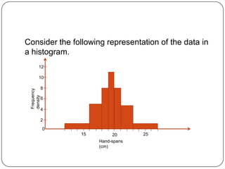
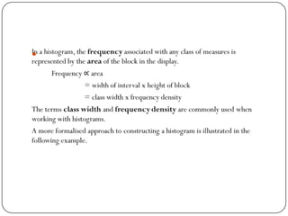
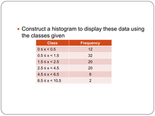
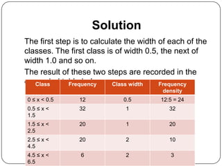
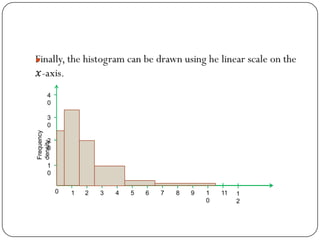
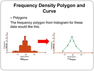
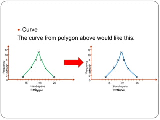
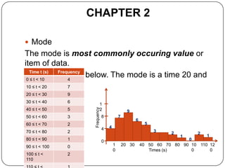
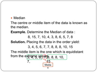
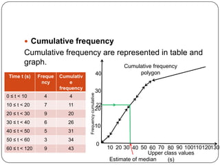
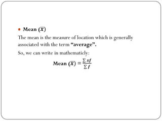
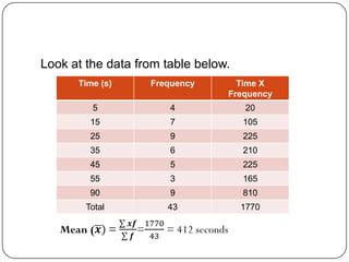
The document discusses histograms, frequency polygons, and other statistical concepts. It provides an example of children's hand span data displayed in a histogram with class intervals. It also shows how to construct a frequency polygon from the histogram and develop a curve from the polygon. Additionally, it defines statistical terms like mode, median, and cumulative frequency and provides examples of calculating each from sets of data.

1. STATISTIC

2. Outline
1. HISTOGRAM
 Histogram
Frequency Density Polygon and Curve
 Polygon
 Curve
2. CHAPTER 2
 Mode
 Median
 Cumulative frequency
 Mean

3. HISTOGRAM
A histogram is a means of displaying continuous data graphically,
conveying the general characteristics data
 The data shown in the display record the hand-spans, in centimetres of a group
of 55 children.
12 0
13
14 5
15 2 5
16 0 1 2 3 4 7
17 0 2 5 9
18 1 2 4 5 6 6 7 8
19 0 2 2 4 5 5 6 8 8 8 9
20 0 2 4 5 6 7 8 9
21 2 3 6 6 7
22 0 1 2 8
23
24 2
25
26 2 5 9

4.  Consider the following representation of the data
in tabulation.
Class Frequency Class Width Frequency
Density
12 ≤ x < 16 4 4 1
16 ≤ x < 18 10 2 5
18 ≤ x < 19 8 1 8
19 ≤ x < 20 11 1 11
20 ≤ x < 21 8 1 8
21 ≤ x < 23 9 2 4,5
23 ≤ x < 27 4 4 1

5. Consider the following representation of the data in
a histogram.
12
10
8
Frequency
density
6
4
2
0
15 20 25
Hand-spans
(cm)

6. 

7.  Construct a histogram to display these data using
the classes given
Class Frequency
0 ≤ x < 0.5 12
0.5 ≤ x < 1.5 32
1.5 ≤ x < 2.5 20
2.5 ≤ x < 4.5 20
4.5 ≤ x < 6.5 6
6.5 ≤ x < 10.5 2

8. Solution
The first step is to calculate the width of each of the
classes. The first class is of width 0.5, the next of
width 1.0 and so on.
The result of these two steps are recorded in the
expanded table below. Class width
Class Frequency Frequency
density
0 ≤ x < 0.5 12 0.5 12:5 = 24
0.5 ≤ x < 32 1 32
1.5
1.5 ≤ x < 20 1 20
2.5
2.5 ≤ x < 20 2 10
4.5
4.5 ≤ x < 6 2 3
6.5

9. 
4
0
3
0
Frequency
2
density
0
1
0
0 1 2 3 4 5 6 7 8 9 1 11 1
0 2

10. Frequency Density Polygon and
Curve
 Polygons
The frequency polygon from histogram for these
data would like this.
12 12
10 10
8 8
Frequency
Frequency
6 6
density
density
4 4
2 2
0 0
15 20 25 15 20 25
Hand-spans Hand-spans
(cm) (cm)
Histogram Polygon

11.  Curve
The curve from polygon above would like this.
12 12
10 10
8 8
Frequency
Frequency
6 6
density
density
4 4
2 2
0 0
15 20 25 15 20 25
Hand-spans Hand-spans
(cm)
Polygon (cm)
Curve

12. CHAPTER 2
 Mode
The mode is most commonly occuring value or
item of data.
Look (s) the data below. The mode is a time 20 and
Time t
0 ≤ t < 10
at Frequency
4
30 tseconds.7
10 ≤ < 20
20 ≤ t < 30 9
30 ≤ t < 40 6
1
40 ≤ t < 50
Frequency
5 2 9
50 ≤ t < 60 3 8 7
6
60 ≤ t < 70 2 5
4 4
70 ≤ t < 80 2 3 2 2
1 1
80 ≤ t < 90 1 0 0
90 ≤ t < 100 0 1 20 30 40 50 60 70 80 90 10 110 12
0 Times (s) 0 0
100 ≤ t < 2
110

13.  Median
The centre or middle item of the data is known as
the median.
Example. Determine the Median of data :
8, 15, 7, 10, 4, 3, 8, 6, 5, 7, 8
Solution. Placing the data in the order yield:
3, 4, 5, 6, 7, 7, 8, 8, 8, 10, 15
The middle item is the one which is equidistant
from the extreme values. 8, 8, 10,
3, 4, 5, 6, 7 ,8,
7, 15
Media
n

14.  Cumulative frequency
Cumulative frequency are represented in table and
graph. Cumulative frequency
40 polygon
Time t (s) Freque Cumulativ
ncy e
frequency
Frequency cumulative 30
0 ≤ t < 10 4 4
10 ≤ t < 20 7 11 22
20
20 ≤ t < 30 9 20
30 ≤ t < 40 6 26
10
40 ≤ t < 50 5 31
50 ≤ t < 60 3 34
0
60 ≤ t < 120 9 43 10 20 30 40 50 60 70 80 90 100110120130
Upper class values
Estimate of median (s)

15. 

16. Look at the data from table below.
Time (s) Frequency Time X
Frequency
5 4 20
15 7 105
25 9 225
35 6 210
45 5 225
55 3 165
90 9 810
Total 43 1770