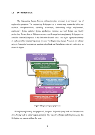
1.0      INTRODUCTION


         The Engineering Design Process outlines the steps necessary in solving any type of
engineering problems. The engineering design process is a multi-step process including the
research, conceptualization, feasibility assessment, establishing design requirements,
preliminary design, detailed design, production planning and tool design, and finally
production. The sections to follow are not necessarily steps in the engineering design process,
for some tasks are completed at the same time as other tasks. This is just a general summary
of each part of the engineering design process. The Engineering Design Process is not a linear
process. Successful engineering requires going back and forth between the six main steps as
shown in Figure 1.


                               Figure 1 Engineering design process


      During the engineering design process, designers frequently jump back and forth between
steps. Going back to earlier steps is common. This way of working is called iteration, and it is
likely that our process will do the same.


                                               1
In this project, we have to use the finite element method (FEM). Its practical application
often known as finite element analysis (FEA)) which is a numerical technique for finding
approximate solutions to partial differential equations (PDE) and their systems, as well as
(less often) integral equations. In simple terms, FEM is a method for dividing up a very
complicated problem into small elements that can be solved in relation to each other. FEM is
a special case of the more general Galerkin method with polynomial approximation
functions. The solution approach is based on eliminating the spatial derivatives from the
PDE. This approximates the PDE with

   a system of algebraic equations for steady state problems,
   a system of ordinary differential equations for transient problems.

    These equation systems are linear if the underlying PDE is linear, and vice versa.
Algebraic equation systems are solved using numerical linear algebra methods. Ordinary
differential equations that arise in transient problems are then numerically integrated using
standard techniques such asEuler's method or the Runge-Kutta method.

    In solving partial differential equations, the primary challenge is to create an equation
that approximates the equation to be studied, but is numerically stable, meaning that errors in
the input and intermediate calculations do not accumulate and cause the resulting output to be
meaningless. There are many ways of doing this, all with advantages and disadvantages. The
finite element method is a good choice for solving partial differential equations over
complicated domains (like cars and oil pipelines), when the domain changes (as during a
solid state reaction with a moving boundary), when the desired precision varies over the
entire domain, or when the solution lacks smoothness. For instance, in a frontal crash
simulation it is possible to increase prediction accuracy in "important" areas like the front of
the car and reduce it in its rear (thus reducing cost of the simulation). Another example would
be in Numerical weather prediction, where it is more important to have accurate predictions
over developing highly nonlinear phenomena (such as tropical cyclones in the atmosphere,
or eddies in the ocean) rather than relatively calm areas.


                                                2
2.0   MODEL DESCRIPTION


      2.1   TASK 1


            3D CAD model as the dimension A = 25mm, B= 20mm, w= 1500 N/m ,
            Poisson’s Ratio (v) = 0.29, Em = 200GPa, Es= 400MPa


                                        Figure 2 Original Beam


                                          Figure 3 Design 1


                                           3
Figure 4 Design 2


Figure 5 Design 3


4
2.2   ANALYSIS

       ORIGINAL BEAM (3D)


                     Figure 6 Deformation of original beam


                             Figure 7 Von-mises stress


                                 5
Figure 8 Translational displacement


     Figure 9 Principle stress


         6
Figure 10 Max & min nodal of Von-mises


Figure 11 Max & min nodal of translational displacement


                   7
Figure 12 Max & min nodal of principle stress


            Original Beam


                     MESH:


            Entity      Size

            Nodes        256

           Elements      771


             ELEMENT TYPE:


       Connectivity       Statistics

           TE4         771 ( 100.00% )


                 8
ELEMENT QUALITY:


          Criterion           Good               Poor           Bad       Worst   Average

                              771 (
           Stretch                            0 ( 0.00% )   0 ( 0.00% )   0.410    0.587
                            100.00% )

                              771 (
         Aspect Ratio                         0 ( 0.00% )   0 ( 0.00% )   3.865    2.234
                            100.00% )


                                              Materials.1


                           Material                          Steel

                      Young's modulus                     2e+011N_m2

                        Poisson's ratio                      0.29

                           Density                        7860kg_m3

            Coefficient of thermal expansion            1.17e-005_Kdeg

                        Yield strength                    4e+008N_m2


                                          Static Case


                                      Boundary Conditions


                                               Figure 1

                                 STRUCTURE Computation

Number of nodes                  : 256
Number of elements               : 771
Number of D.O.F.                 : 768
Number of Contact relations      : 0
Number of Kinematic relations    : 0


Linear tetrahedron : 771
                                          9
RESTRAINT Computation

 Name: Restraints.1

 Number of S.P.C : 90

                               LOAD Computation

 Name: Loads.1

 Applied load resultant :


                             STIFFNESS Computation

Number of lines                                : 768
Number of coefficients                         : 12642
Number of blocks                               :     1
Maximum number of coefficients per bloc        : 12642
Total matrix size                              :     0 . 15 Mb


                            SINGULARITY Computation

Restraint: Restraints.1

Number of local singularities               :   0
Number of singularities in translation      :   0
Number of singularities in rotation         :   0
Generated constraint type                   : MPC


                            CONSTRAINT Computation

Restraint: Restraints.1

Number of constraints              :   90
Number of coefficients             :    0
Number of factorized constraints   :   90
Number of coefficients             :    0
Number of deferred constraints     :    0


                            FACTORIZED Computation

Method                                 :     SPARSE
Number of factorized degrees           : 678
Number of supernodes                   : 135
Number of overhead indices             : 3954
Number of coefficients                 : 26211
Maximum front width                    :    72
Maximum front size                     : 2628


                                              10
Size of the factorized matrix (Mb)     :      0   . 199974
    Number of blocks                       :      1
    Number of Mflops for factorization     :      1   . 356e+000
    Number of Mflops for solve             :      1   . 082e-001
    Minimum relative pivot                 :      2   . 764e-002

    Minimum and maximum pivot


       Value        Dof    Node          x (mm)           y (mm)        z (mm)

    2.8078e+008      Tx     256        5.5259e+000      6.5176e+000   2.6446e+001

    1.2646e+010      Ty     221        1.4819e+001      5.8076e+000   1.1835e+002


    Minimum pivot


       Value        Dof    Node          x (mm)           y (mm)        z (mm)

    3.1157e+008      Ty     256        5.5259e+000      6.5176e+000   2.6446e+001

    8.5879e+008      Ty     240        8.8304e+000      1.2999e+001   1.0319e+002

    8.8355e+008      Tz     225        1.0611e+001      1.9616e+001   5.6535e+001

    8.8865e+008      Tx     244        6.1865e+000      5.9668e+000   8.2072e+001

    8.9038e+008      Tz     243        1.0395e+001      1.3270e+001   9.3997e+001

    8.9809e+008      Tz     226        1.0087e+001      1.9574e+001   6.5662e+001

    9.0152e+008      Ty     251        1.0388e+001      1.3258e+001   5.6463e+001

    9.0499e+008      Tx     227        9.4759e+000      1.9519e+001   7.4732e+001

    9.1072e+008      Tx     226        1.0087e+001      1.9574e+001   6.5662e+001


    Translational pivot distribution


          Value           Percentage

     10.E8 --> 10.E9      3.0973e+000

    10.E9 --> 10.E10      9.6313e+001

    10.E10 --> 10.E11     5.8997e-001


                            DIRECT METHOD Computation

Name: Static Case Solution.1

Restraint: Restraints.1

Load: Loads.1

Strain Energy : 2.495e-005 J

                                               11
Equilibrium


                         Applied                                                 Relative
   Components                                Reactions         Residual
                         Forces                                               Magnitude Error

      Fx (N)             -2.2500e+002          2.2500e+002     9.9476e-013           2.3287e-014

      Fy (N)              -2.4980e-014          8.9084e-013    8.6586e-013           2.0270e-014

      Fz (N)              4.5157e-014           7.1487e-013    7.6003e-013           1.7792e-014

    Mx (Nxm)              -1.0037e-014         -7.6279e-014    -8.6316e-014          1.3471e-014

    My (Nxm)             -1.6875e+001          1.6875e+001     1.5277e-013           2.3842e-014

    Mz (Nxm)              2.8125e+000          -2.8125e+000    5.0626e-014           7.9011e-015


                         Static Case Solution.1 - Deformed mesh.2


                                                    Figure 2

On deformed mesh ---- On boundary ---- Over all the model


                                          12
Static Case Solution.1 - Von Mises stress (nodal values).2


                                            Figure 3

3D elements: : Components: : All

On deformed mesh ---- On boundary ---- Over all the model

                                     Global Sensors


                             Sensor Name         Sensor Value

                                   Energy          2.495e-005J


                                              13
2.3   TASK 2


       DESIGN 1


                          Figure 13 Design 1


                   Figure 14 Deformation of Design 1


                              14
Figure 15 Von-mises stress of Design 1


Figure 16 Translational displacement of Design 1


                  15
Figure 17 Principle stress of Design 1


 DESIGN 2


                        Figure 18 Design 2


                          16
Figure 19 Deformation of Design 2


Figure 20 Von-mises stress of Design 2


             17
Figure 21 Translational displacement of Design 2


     Figure 22 Principle stress of Design 2


                  18
 DESIGN 3


                    Figure 23 Design 3


             Figure 24 Deformation of Design 3


                        19
Figure 25 Von-mises stress of Design 3


Figure 26 Translational displacement of Design 3


                  20
Figure 27 Principle stress of Design 3


             21
2.4       MORPHOLOGICAL CHART


  DESIGN          Original beam   Design 1   Design 2   Design 3


A (mm)                 25           25         25         25

B (mm)                 20           20         20         20

w (N/m)               1500         1500       1500       1500

Poisson’s             0.29          0.29       0.29       0.29
ratio (v)
Em (GPa)              200           200        200        200
Es (MPa)              400           400        400        400

Von Misses          8.32x10⁷      9.89x10⁷   2.82x10⁷   1.26x10⁷
Stress (Nm2)
Translational       0.000426      0.000507   0.000644   0.000277
Displacement
(mm)
Principal           1.09x10⁷      1.31x10⁷   1.91x10⁷   1.07x10⁷
Stress (Nm2)


                                    22
3.0    DISCUSSION


       From the analysis above, I had done the finite element analysis (FEA) for original
just in 3D. The Von-Mises Stress obtained is 8.32 x10⁷ Nm2 , Translational displacement is
0.000426 mm, and Principle Stress is 1.09x10⁷ Nm2 for 3D beam by using CATIA.


       A beam is a structural element that is capable of withstanding load primarily by
resisting bending. The bending force induced into the material of the beam as a result of the
external loads, own weight, span and external reactions to these loads is called a bending
moment. In order to increase the stiffness of the bracket without compromising the
dimensions, we have to design 3 concepts to overcome the problem. However, only one out
from three of my design was successfully done. By increasing the stiffness of the beam, the
deflection of the rectangular support bracket must be reduced.


       From the result obtained, the 1st design introduced us a poor result than the original
beam. The value of Von Misses Stress = 9.89x10⁷ Nm2, Translational Displacement =
0.000507 mm and Principal Stress= 1.31x10⁷Nm2. All the value is much greater than the
original beam, thus this design cannot promote to increase the stiffness of the bracket.


       For the 2nd design, the value of the Von Misses Stress = 2.82x10⁷ Nm2, Translational
Displacement = 0.000644 mm and Principal Stress = 1.91x107x107 Nm2. This design also
gives the poor result than the original beam and design 1.


       However, the third design was successfully obtained the exact value to increase the
stiffness due to its value for Von Misses Stress = 1.26 x10⁷ Nm2, Translational
Displacement = 0.000277 mm and Principal Stress = 1.07x10⁷ Nm2. This design is the best
among the other design because have less value than the original beam. So, this design can
be promote to increase the stiffness and reduced the deflection.


                                              23
4.0    CONCLUSIONS


       As the conclusion, based on the translational displacement, the best design goes to the
 rd
3 design; where the translational displacement of the beam is smaller than the original beam
which is 0.000277 mm rather than 0.000426 mm. Thus this design can overcome the
problem.


5.0    APPENDIX


       (a)      ADDITIONAL STRESS CONTOUR PLOT


       The program provides two types of stress contour plots: a von Mises-Hencky effective
       stress plot and a Factor of Safety on Material Yield plot. In both of these plots the
       maximum stress plotted is limited to the yield strength of the cable component. Thus,
       where stress concentrations occur, the maximum stress reported by the program will
       never exceed the yield strength.

       The following stress contours are available:

             1. Stress xx -      contour;
             2. Stress yy -      contour;
             3. Stress xy -     contour;
             4. Stress zz -     contour;
             5. Major Principal -      contour;
             6. Minor Principal -      contour;

             7. Stress 1/ Stress 3 -       contour;
             8. Max. Shear -         contour;
             9. P - mean stress.                            contour;

             10. q - shear stress.                    is the second stress invariants;
             11. q/p - ratio of q/p as defined above;
             12. Pore pressure - pore water pressure;
             13. Yield zone - PISA actually plots the the value of the yield zone function f for
                 plastic models.


                                                  24
(b)     REFERENCES


   i.   http://en.wikipedia.org/wiki/Beam_(structure)
 ii.    http://en.wikipedia.org/wiki/Finite_element_analysis
 iii.   http://answers.yahoo.com/question/index?qid=20081120131225AAbKEvM
 iv.    http://www.newport.com/Fundamentals-of
        Vibration/140234/1033/content.aspx
  v.    http://cedb.asce.org/cgi/WWWdisplay.cgi?115570


                                      25

CAE REPORT

  • 1.
    1.0 INTRODUCTION The Engineering Design Process outlines the steps necessary in solving any type of engineering problems. The engineering design process is a multi-step process including the research, conceptualization, feasibility assessment, establishing design requirements, preliminary design, detailed design, production planning and tool design, and finally production. The sections to follow are not necessarily steps in the engineering design process, for some tasks are completed at the same time as other tasks. This is just a general summary of each part of the engineering design process. The Engineering Design Process is not a linear process. Successful engineering requires going back and forth between the six main steps as shown in Figure 1. Figure 1 Engineering design process During the engineering design process, designers frequently jump back and forth between steps. Going back to earlier steps is common. This way of working is called iteration, and it is likely that our process will do the same. 1
  • 2.
    In this project,we have to use the finite element method (FEM). Its practical application often known as finite element analysis (FEA)) which is a numerical technique for finding approximate solutions to partial differential equations (PDE) and their systems, as well as (less often) integral equations. In simple terms, FEM is a method for dividing up a very complicated problem into small elements that can be solved in relation to each other. FEM is a special case of the more general Galerkin method with polynomial approximation functions. The solution approach is based on eliminating the spatial derivatives from the PDE. This approximates the PDE with  a system of algebraic equations for steady state problems,  a system of ordinary differential equations for transient problems. These equation systems are linear if the underlying PDE is linear, and vice versa. Algebraic equation systems are solved using numerical linear algebra methods. Ordinary differential equations that arise in transient problems are then numerically integrated using standard techniques such asEuler's method or the Runge-Kutta method. In solving partial differential equations, the primary challenge is to create an equation that approximates the equation to be studied, but is numerically stable, meaning that errors in the input and intermediate calculations do not accumulate and cause the resulting output to be meaningless. There are many ways of doing this, all with advantages and disadvantages. The finite element method is a good choice for solving partial differential equations over complicated domains (like cars and oil pipelines), when the domain changes (as during a solid state reaction with a moving boundary), when the desired precision varies over the entire domain, or when the solution lacks smoothness. For instance, in a frontal crash simulation it is possible to increase prediction accuracy in "important" areas like the front of the car and reduce it in its rear (thus reducing cost of the simulation). Another example would be in Numerical weather prediction, where it is more important to have accurate predictions over developing highly nonlinear phenomena (such as tropical cyclones in the atmosphere, or eddies in the ocean) rather than relatively calm areas. 2
  • 3.
    2.0 MODEL DESCRIPTION 2.1 TASK 1 3D CAD model as the dimension A = 25mm, B= 20mm, w= 1500 N/m , Poisson’s Ratio (v) = 0.29, Em = 200GPa, Es= 400MPa Figure 2 Original Beam Figure 3 Design 1 3
  • 4.
    Figure 4 Design2 Figure 5 Design 3 4
  • 5.
    2.2 ANALYSIS  ORIGINAL BEAM (3D) Figure 6 Deformation of original beam Figure 7 Von-mises stress 5
  • 6.
    Figure 8 Translationaldisplacement Figure 9 Principle stress 6
  • 7.
    Figure 10 Max& min nodal of Von-mises Figure 11 Max & min nodal of translational displacement 7
  • 8.
    Figure 12 Max& min nodal of principle stress Original Beam MESH: Entity Size Nodes 256 Elements 771 ELEMENT TYPE: Connectivity Statistics TE4 771 ( 100.00% ) 8
  • 9.
    ELEMENT QUALITY: Criterion Good Poor Bad Worst Average 771 ( Stretch 0 ( 0.00% ) 0 ( 0.00% ) 0.410 0.587 100.00% ) 771 ( Aspect Ratio 0 ( 0.00% ) 0 ( 0.00% ) 3.865 2.234 100.00% ) Materials.1 Material Steel Young's modulus 2e+011N_m2 Poisson's ratio 0.29 Density 7860kg_m3 Coefficient of thermal expansion 1.17e-005_Kdeg Yield strength 4e+008N_m2 Static Case Boundary Conditions Figure 1 STRUCTURE Computation Number of nodes : 256 Number of elements : 771 Number of D.O.F. : 768 Number of Contact relations : 0 Number of Kinematic relations : 0 Linear tetrahedron : 771 9
  • 10.
    RESTRAINT Computation Name:Restraints.1 Number of S.P.C : 90 LOAD Computation Name: Loads.1 Applied load resultant : STIFFNESS Computation Number of lines : 768 Number of coefficients : 12642 Number of blocks : 1 Maximum number of coefficients per bloc : 12642 Total matrix size : 0 . 15 Mb SINGULARITY Computation Restraint: Restraints.1 Number of local singularities : 0 Number of singularities in translation : 0 Number of singularities in rotation : 0 Generated constraint type : MPC CONSTRAINT Computation Restraint: Restraints.1 Number of constraints : 90 Number of coefficients : 0 Number of factorized constraints : 90 Number of coefficients : 0 Number of deferred constraints : 0 FACTORIZED Computation Method : SPARSE Number of factorized degrees : 678 Number of supernodes : 135 Number of overhead indices : 3954 Number of coefficients : 26211 Maximum front width : 72 Maximum front size : 2628 10
  • 11.
    Size of thefactorized matrix (Mb) : 0 . 199974 Number of blocks : 1 Number of Mflops for factorization : 1 . 356e+000 Number of Mflops for solve : 1 . 082e-001 Minimum relative pivot : 2 . 764e-002 Minimum and maximum pivot Value Dof Node x (mm) y (mm) z (mm) 2.8078e+008 Tx 256 5.5259e+000 6.5176e+000 2.6446e+001 1.2646e+010 Ty 221 1.4819e+001 5.8076e+000 1.1835e+002 Minimum pivot Value Dof Node x (mm) y (mm) z (mm) 3.1157e+008 Ty 256 5.5259e+000 6.5176e+000 2.6446e+001 8.5879e+008 Ty 240 8.8304e+000 1.2999e+001 1.0319e+002 8.8355e+008 Tz 225 1.0611e+001 1.9616e+001 5.6535e+001 8.8865e+008 Tx 244 6.1865e+000 5.9668e+000 8.2072e+001 8.9038e+008 Tz 243 1.0395e+001 1.3270e+001 9.3997e+001 8.9809e+008 Tz 226 1.0087e+001 1.9574e+001 6.5662e+001 9.0152e+008 Ty 251 1.0388e+001 1.3258e+001 5.6463e+001 9.0499e+008 Tx 227 9.4759e+000 1.9519e+001 7.4732e+001 9.1072e+008 Tx 226 1.0087e+001 1.9574e+001 6.5662e+001 Translational pivot distribution Value Percentage 10.E8 --> 10.E9 3.0973e+000 10.E9 --> 10.E10 9.6313e+001 10.E10 --> 10.E11 5.8997e-001 DIRECT METHOD Computation Name: Static Case Solution.1 Restraint: Restraints.1 Load: Loads.1 Strain Energy : 2.495e-005 J 11
  • 12.
    Equilibrium Applied Relative Components Reactions Residual Forces Magnitude Error Fx (N) -2.2500e+002 2.2500e+002 9.9476e-013 2.3287e-014 Fy (N) -2.4980e-014 8.9084e-013 8.6586e-013 2.0270e-014 Fz (N) 4.5157e-014 7.1487e-013 7.6003e-013 1.7792e-014 Mx (Nxm) -1.0037e-014 -7.6279e-014 -8.6316e-014 1.3471e-014 My (Nxm) -1.6875e+001 1.6875e+001 1.5277e-013 2.3842e-014 Mz (Nxm) 2.8125e+000 -2.8125e+000 5.0626e-014 7.9011e-015 Static Case Solution.1 - Deformed mesh.2 Figure 2 On deformed mesh ---- On boundary ---- Over all the model 12
  • 13.
    Static Case Solution.1- Von Mises stress (nodal values).2 Figure 3 3D elements: : Components: : All On deformed mesh ---- On boundary ---- Over all the model Global Sensors Sensor Name Sensor Value Energy 2.495e-005J 13
  • 14.
    2.3 TASK 2  DESIGN 1 Figure 13 Design 1 Figure 14 Deformation of Design 1 14
  • 15.
    Figure 15 Von-misesstress of Design 1 Figure 16 Translational displacement of Design 1 15
  • 16.
    Figure 17 Principlestress of Design 1  DESIGN 2 Figure 18 Design 2 16
  • 17.
    Figure 19 Deformationof Design 2 Figure 20 Von-mises stress of Design 2 17
  • 18.
    Figure 21 Translationaldisplacement of Design 2 Figure 22 Principle stress of Design 2 18
  • 19.
     DESIGN 3 Figure 23 Design 3 Figure 24 Deformation of Design 3 19
  • 20.
    Figure 25 Von-misesstress of Design 3 Figure 26 Translational displacement of Design 3 20
  • 21.
    Figure 27 Principlestress of Design 3 21
  • 22.
    2.4 MORPHOLOGICAL CHART DESIGN Original beam Design 1 Design 2 Design 3 A (mm) 25 25 25 25 B (mm) 20 20 20 20 w (N/m) 1500 1500 1500 1500 Poisson’s 0.29 0.29 0.29 0.29 ratio (v) Em (GPa) 200 200 200 200 Es (MPa) 400 400 400 400 Von Misses 8.32x10⁷ 9.89x10⁷ 2.82x10⁷ 1.26x10⁷ Stress (Nm2) Translational 0.000426 0.000507 0.000644 0.000277 Displacement (mm) Principal 1.09x10⁷ 1.31x10⁷ 1.91x10⁷ 1.07x10⁷ Stress (Nm2) 22
  • 23.
    3.0 DISCUSSION From the analysis above, I had done the finite element analysis (FEA) for original just in 3D. The Von-Mises Stress obtained is 8.32 x10⁷ Nm2 , Translational displacement is 0.000426 mm, and Principle Stress is 1.09x10⁷ Nm2 for 3D beam by using CATIA. A beam is a structural element that is capable of withstanding load primarily by resisting bending. The bending force induced into the material of the beam as a result of the external loads, own weight, span and external reactions to these loads is called a bending moment. In order to increase the stiffness of the bracket without compromising the dimensions, we have to design 3 concepts to overcome the problem. However, only one out from three of my design was successfully done. By increasing the stiffness of the beam, the deflection of the rectangular support bracket must be reduced. From the result obtained, the 1st design introduced us a poor result than the original beam. The value of Von Misses Stress = 9.89x10⁷ Nm2, Translational Displacement = 0.000507 mm and Principal Stress= 1.31x10⁷Nm2. All the value is much greater than the original beam, thus this design cannot promote to increase the stiffness of the bracket. For the 2nd design, the value of the Von Misses Stress = 2.82x10⁷ Nm2, Translational Displacement = 0.000644 mm and Principal Stress = 1.91x107x107 Nm2. This design also gives the poor result than the original beam and design 1. However, the third design was successfully obtained the exact value to increase the stiffness due to its value for Von Misses Stress = 1.26 x10⁷ Nm2, Translational Displacement = 0.000277 mm and Principal Stress = 1.07x10⁷ Nm2. This design is the best among the other design because have less value than the original beam. So, this design can be promote to increase the stiffness and reduced the deflection. 23
  • 24.
    4.0 CONCLUSIONS As the conclusion, based on the translational displacement, the best design goes to the rd 3 design; where the translational displacement of the beam is smaller than the original beam which is 0.000277 mm rather than 0.000426 mm. Thus this design can overcome the problem. 5.0 APPENDIX (a) ADDITIONAL STRESS CONTOUR PLOT The program provides two types of stress contour plots: a von Mises-Hencky effective stress plot and a Factor of Safety on Material Yield plot. In both of these plots the maximum stress plotted is limited to the yield strength of the cable component. Thus, where stress concentrations occur, the maximum stress reported by the program will never exceed the yield strength. The following stress contours are available: 1. Stress xx - contour; 2. Stress yy - contour; 3. Stress xy - contour; 4. Stress zz - contour; 5. Major Principal - contour; 6. Minor Principal - contour; 7. Stress 1/ Stress 3 - contour; 8. Max. Shear - contour; 9. P - mean stress. contour; 10. q - shear stress. is the second stress invariants; 11. q/p - ratio of q/p as defined above; 12. Pore pressure - pore water pressure; 13. Yield zone - PISA actually plots the the value of the yield zone function f for plastic models. 24
  • 25.
    (b) REFERENCES i. http://en.wikipedia.org/wiki/Beam_(structure) ii. http://en.wikipedia.org/wiki/Finite_element_analysis iii. http://answers.yahoo.com/question/index?qid=20081120131225AAbKEvM iv. http://www.newport.com/Fundamentals-of Vibration/140234/1033/content.aspx v. http://cedb.asce.org/cgi/WWWdisplay.cgi?115570 25