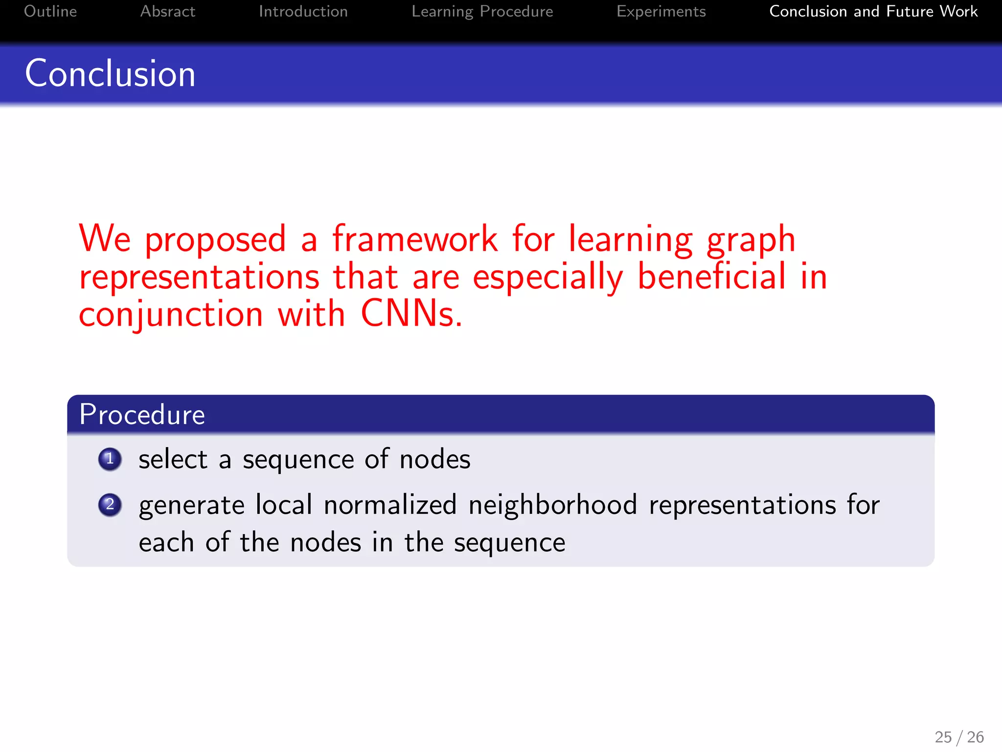
This document summarizes a research paper on learning convolutional neural networks for graphs. It proposes a framework called PATCHY-SAN that applies CNNs to graphs by (1) selecting a node sequence and (2) generating normalized neighborhood representations for each node. Experimental results show PATCHY-SAN achieves accuracy competitive with graph kernels while being 2-8 times more efficient on benchmark graph classification tasks. The document concludes CNNs may be especially beneficial for learning graph representations when used with this proposed framework.

1. Learning Convolutional Neural Networks for Graphs
pione30

2. All of the figures in this presentation are, unless
explicitly stated, those of the original paper1
.
1
http://proceedings.mlr.press/v48/niepert16.pdf

3. Outline Absract Introduction Learning Procedure Experiments Conclusion and Future Work
1 Absract
2 Introduction
3 Learning Procedure
4 Experiments
5 Conclusion and Future Work
3 / 26

4. Outline Absract Introduction Learning Procedure Experiments Conclusion and Future Work
1 Absract
2 Introduction
3 Learning Procedure
4 Experiments
5 Conclusion and Future Work
4 / 26

5. Outline Absract Introduction Learning Procedure Experiments Conclusion and Future Work
Absract
We propose a framework for learning Convolutional Neural
Networks (CNN) for arbitrary graphs.
5 / 26

6. Outline Absract Introduction Learning Procedure Experiments Conclusion and Future Work
Absract
We claim that . . .
the learned feature representations are competitive with state
of the art graph kernels.
computation is highly efficient.
6 / 26

7. Outline Absract Introduction Learning Procedure Experiments Conclusion and Future Work
1 Absract
2 Introduction
3 Learning Procedure
4 Experiments
5 Conclusion and Future Work
7 / 26

8. Outline Absract Introduction Learning Procedure Experiments Conclusion and Future Work
The architecture of CNN
Figure 1: The architecture of CNN2
2
http://cs231n.github.io/convolutional-networks/
8 / 26

9. Outline Absract Introduction Learning Procedure Experiments Conclusion and Future Work
The receptive field and the neighborhood graph of CNN
The locally connected receptive field constructed by the
neighborhood graph is essential for CNN.
9 / 26

10. Outline Absract Introduction Learning Procedure Experiments Conclusion and Future Work
The receptive field and the neighborhood graph of CNN
KONSTANTIN.KUTZKOV@NECLAB.EU
1 2
3 4
1 2
3 4
1 2
3 4
1 2
3 4
1 1 1 1... ...
......(b)
(a)
Figure 1. A CNN with a receptive field of size 3x3. The field is
moved over an image from left to right and top to bottom using a
particular stride (here: 1) and zero-padding (here: none) (a). The
values read by the receptive fields are transformed into a linear
Figure 2: A CNN with a receptive field of size 3x3. The field is moved
over an image from left to right and top to bottom (a). The values read
by the receptive fields can be transformed into a vector representation
(b). 10 / 26

11. Outline Absract Introduction Learning Procedure Experiments Conclusion and Future Work
The receptive field and the neighborhood graph of CNN
CNN for images . . .
Due to the implicit spatial order of the pixels, the sequence of
nodes for which neighborhood graphs are created is uniquely
determined.
11 / 26

12. Outline Absract Introduction Learning Procedure Experiments Conclusion and Future Work
Collection of arbitrary graphs
One has to . . .
1 determine the node sequences for which neighborhood graphs
are created
2 compute a normalization of neighborhood graphs, that is, a
unique mapping from a graph representation into a vector
space representation.
12 / 26

13. Outline Absract Introduction Learning Procedure Experiments Conclusion and Future Work
Collection of arbitrary graphs
One has to . . .
1 determine the node sequences for which neighborhood graphs
are created
2 compute a normalization of neighborhood graphs, that is, a
unique mapping from a graph representation into a vector
space representation.
→ We proposed new approach termed PATCHY-SAN.
12 / 26

14. Outline Absract Introduction Learning Procedure Experiments Conclusion and Future Work
1 Absract
2 Introduction
3 Learning Procedure
4 Experiments
5 Conclusion and Future Work
13 / 26

15. Outline Absract Introduction Learning Procedure Experiments Conclusion and Future Work
The architecture of PATCHY-SAN
onal Neural Networks for Graphs
col-
, or
not
two
hich
nor-
map-
rep-
AN,
each
for
hese
ex-
to a
... ...
neighborhood graph construction
convolutional architecture
node sequence selection
graph normalization
Figure 2. An illustration of the proposed architecture. A node
sequence is selected from a graph via a graph labeling procedure.
For some nodes in the sequence, a local neighborhood graph is as-
sembled and normalized. The normalized neighborhoods are used
Figure 3: An illustration of the PATCHY-SAN architecture.
14 / 26

16. Outline Absract Introduction Learning Procedure Experiments Conclusion and Future Work
Preparation
One has to determine a labeling procedure ℓ which is used to
sort the graph and select a node sequence.
ℓ is also used when normalizing a neighborhood subgraph.
15 / 26

17. Outline Absract Introduction Learning Procedure Experiments Conclusion and Future Work
Architecture
Learning Convolutional Neural Networks for Graphs
4
2
5
3
1
4
21
3
normalize
subgraph
receptive field
reads vertex and edge
attributes = channels
select
neighborhood
... ...
1 2 3 4 5 1 2 3
Figure 3. The normalization is performed for each of the graphs induced on the neighborhood of a root node v (the red node; node
colors indicate distance to the root node). A graph labeling is used to rank the nodes and to create the normalized receptive fields, one of
size k (here: k = 9) for node attributes and one of size k × k for edge attributes. Normalization also includes cropping of excess nodes
and padding with dummy nodes. Each vertex (edge) attribute corresponds to an input channel with the respective receptive field.
Algorithm 3 RECEPTIVEFIELD: Create Receptive Field
1: input: vertex v, graph labeling , receptive field size k
2: N = NEIGHASSEMB(v, k)
3: Gnorm = NORMALIZEGRAPH(N, v, , k)
4: return Gnorm
random from G, the expected difference between the dis-
tance of the graphs in vector space (with respect to the ad-
Algorithm 4 NORMALIZEGRAPH: Graph Normalization
1: input: subset of vertices U from original graph G, vertex v,
graph labeling , receptive field size k
2: output: receptive field for v
3: compute ranking r of U using , subject to
∀u, w ∈ U : d(u, v) < d(w, v) ⇒ r(u) < r(w)
4: if |U| > k then
5: N = top k vertices in U according to r
6: compute ranking r of N using , subject to
Figure 4: The normalization procedure
16 / 26

18. Outline Absract Introduction Learning Procedure Experiments Conclusion and Future Work
1 Absract
2 Introduction
3 Learning Procedure
4 Experiments
5 Conclusion and Future Work
17 / 26

19. Outline Absract Introduction Learning Procedure Experiments Conclusion and Future Work
Runtime Analysis
PATCHY-SAN with 1-dimensional Weisfeiler-Lehman (1-WL)
algorithm for the normalization.
input graphs (graph-tool3collection)
torus
random
power
polbooks
preferential
astro-ph
email-enron
3
https://graph-tool.skewed.de/
18 / 26

20. Outline Absract Introduction Learning Procedure Experiments Conclusion and Future Work
Runtime Analysis
onal Neural Networks for Graphs
size
king
ank-
aller
t in-
s the
ows.
m an
size
mal-
uta-
with
5 10 20 30 40 50
Field size (k)
500
1500
2500
3500
4500
Fields/sec.
torus
random
power
pol-books
preferential
astro-ph
email-enron
Figure 4. Receptive fields per second rates on different graphs.
k. Let d be the maximum degree of the input graph G,
and U the neighborhood returned by Algorithm 2. We have
Figure 5: Receptive fields per second rates on different graphs.
19 / 26

21. Outline Absract Introduction Learning Procedure Experiments Conclusion and Future Work
Runtime Analysis
onal Neural Networks for Graphs
size
king
ank-
aller
t in-
s the
ows.
m an
size
mal-
uta-
with
5 10 20 30 40 50
Field size (k)
500
1500
2500
3500
4500
Fields/sec.
torus
random
power
pol-books
preferential
astro-ph
email-enron
Figure 4. Receptive fields per second rates on different graphs.
k. Let d be the maximum degree of the input graph G,
and U the neighborhood returned by Algorithm 2. We have
Figure 5: Receptive fields per second rates on different graphs.
the speed at which receptive fields are generated is sufficient to
saturate a CNN.
19 / 26

22. Outline Absract Introduction Learning Procedure Experiments Conclusion and Future Work
Graph Classification
Comparison: PATCHY-SAN with . . .
shortest-path kernel (SP)
random walk kernel (RW)
graphlet count kernel (GK)
Weisfeiler-Lehman subtree kernel (WL)
Parameters
The decay factor for RW is chosen from
{10−6, 10−5, . . . , 10−1}
The size of the graphlets for GK is 7
The height parameter of WL is 2
20 / 26

23. Outline Absract Introduction Learning Procedure Experiments Conclusion and Future Work
Graph Classification
Data sets
MUTAG
PCT
NCI1
NCI109
PROTEIN
D&D
21 / 26

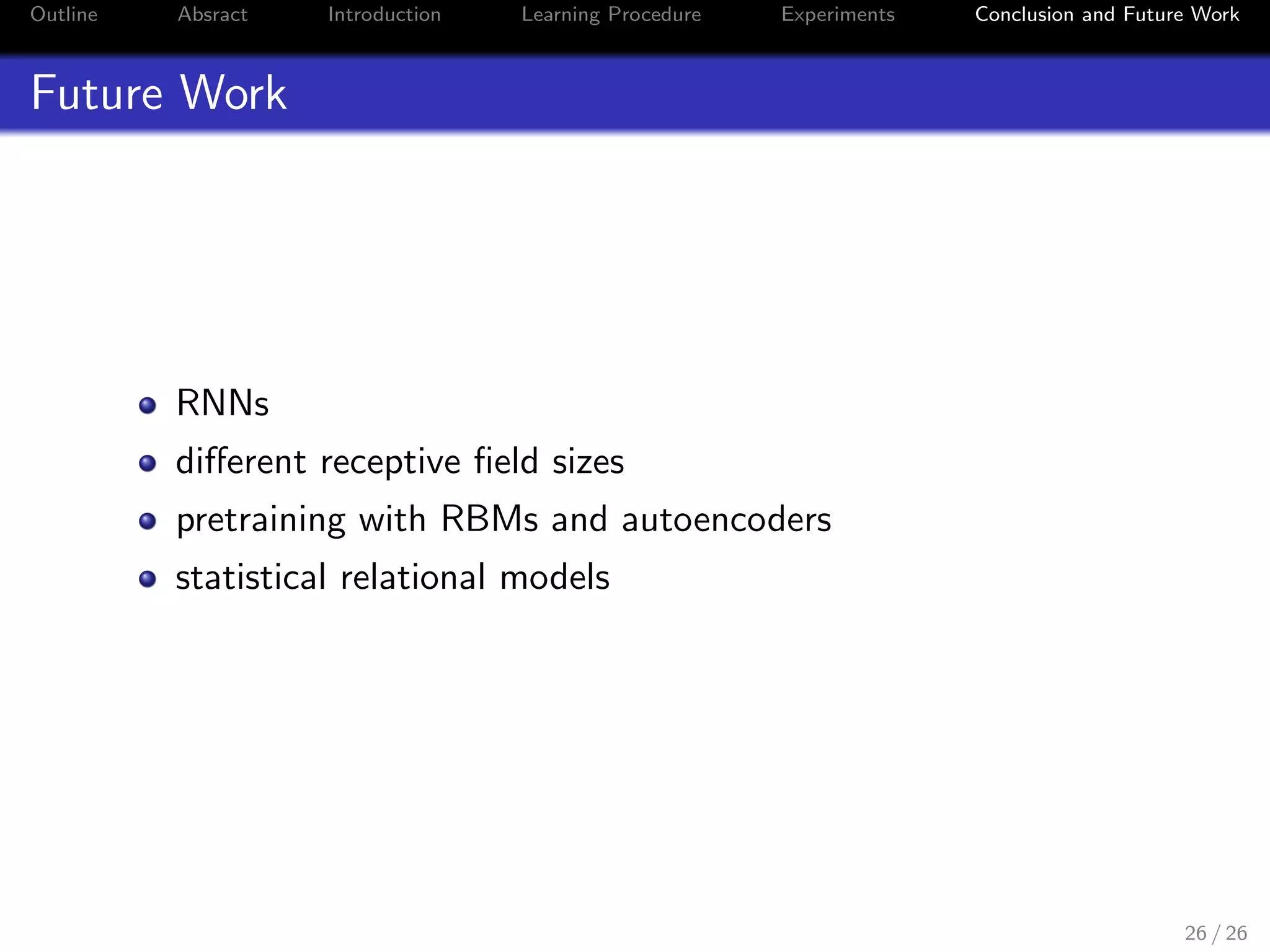
24. Outline Absract Introduction Learning Procedure Experiments Conclusion and Future Work
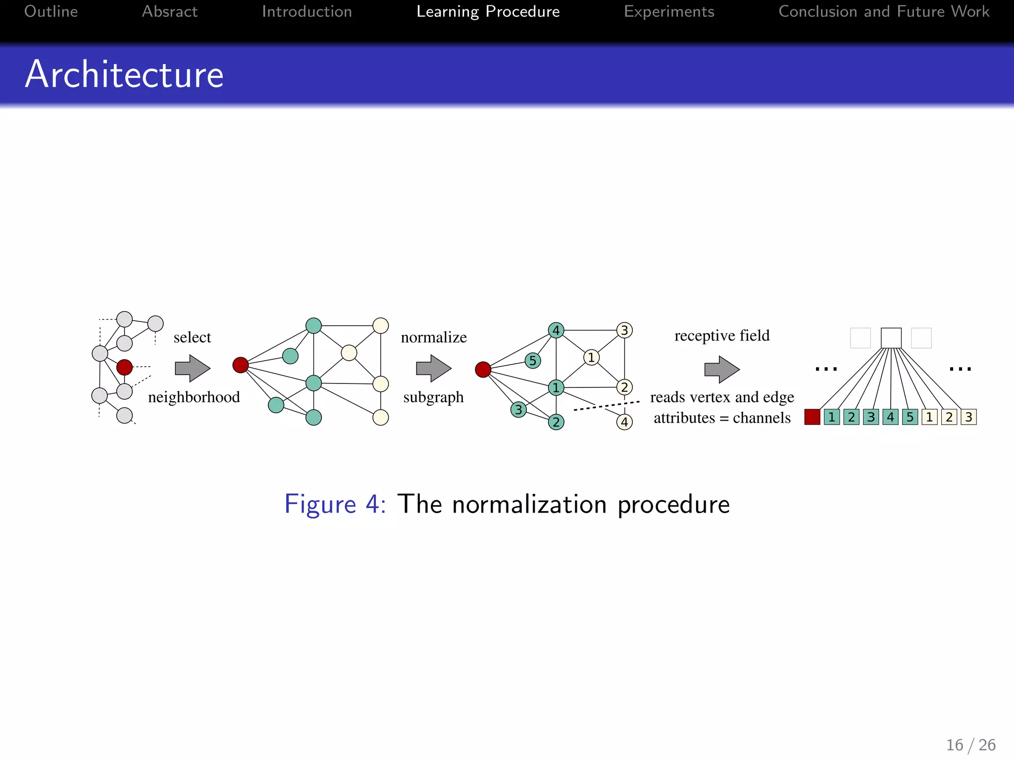
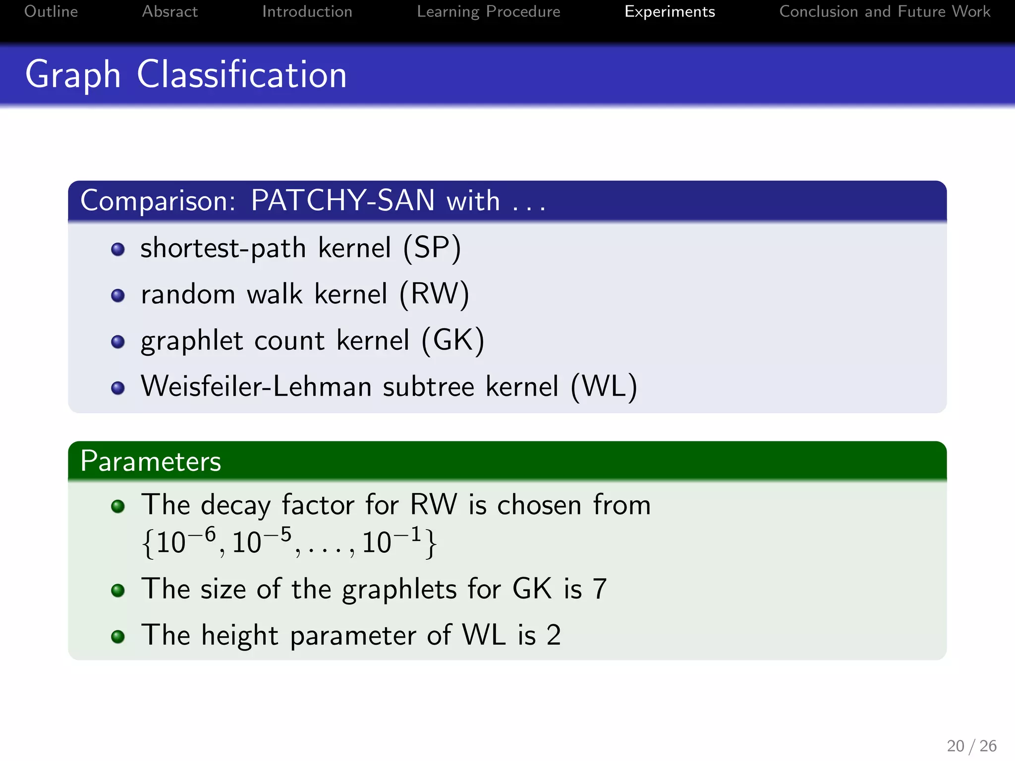
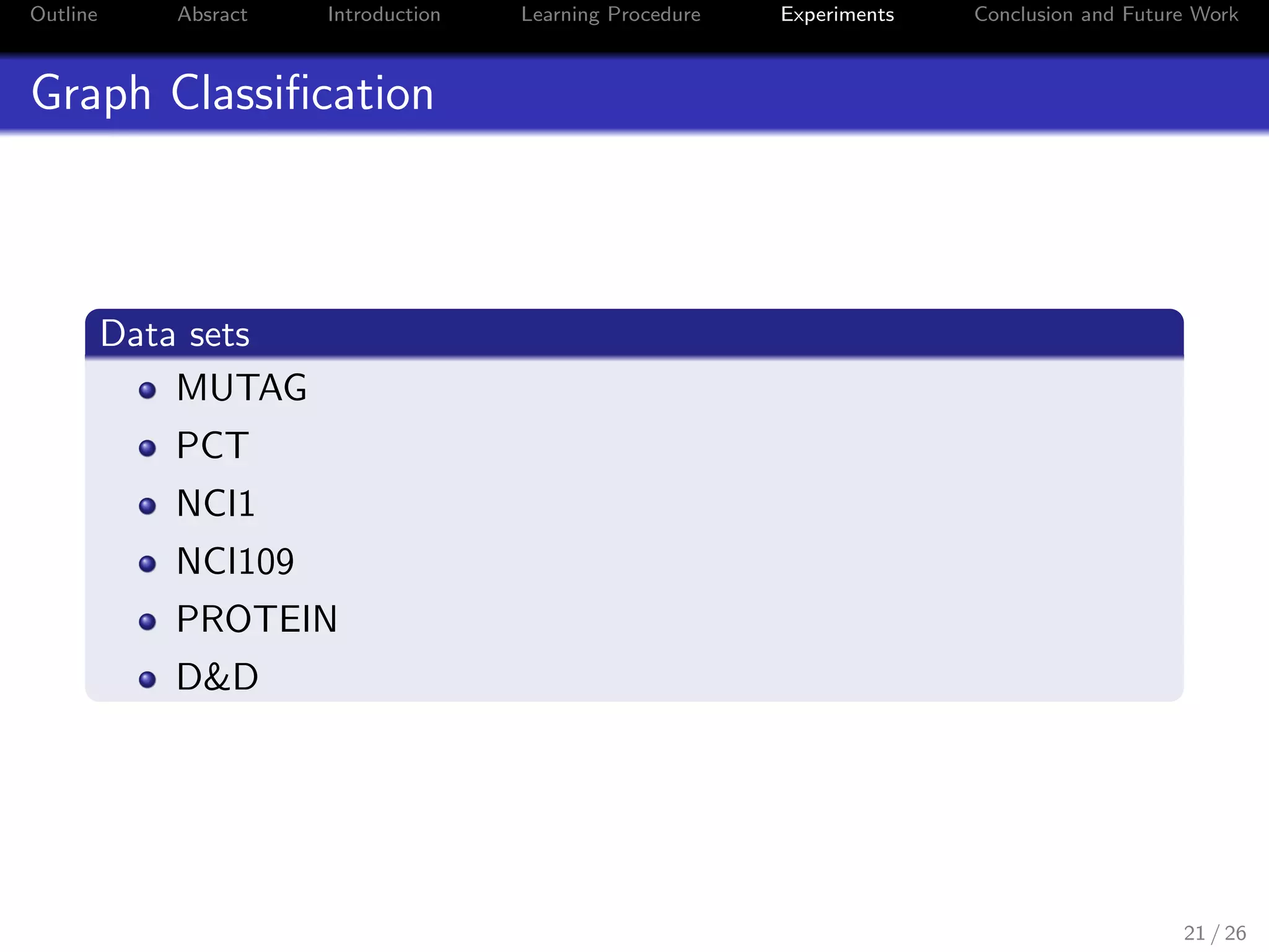
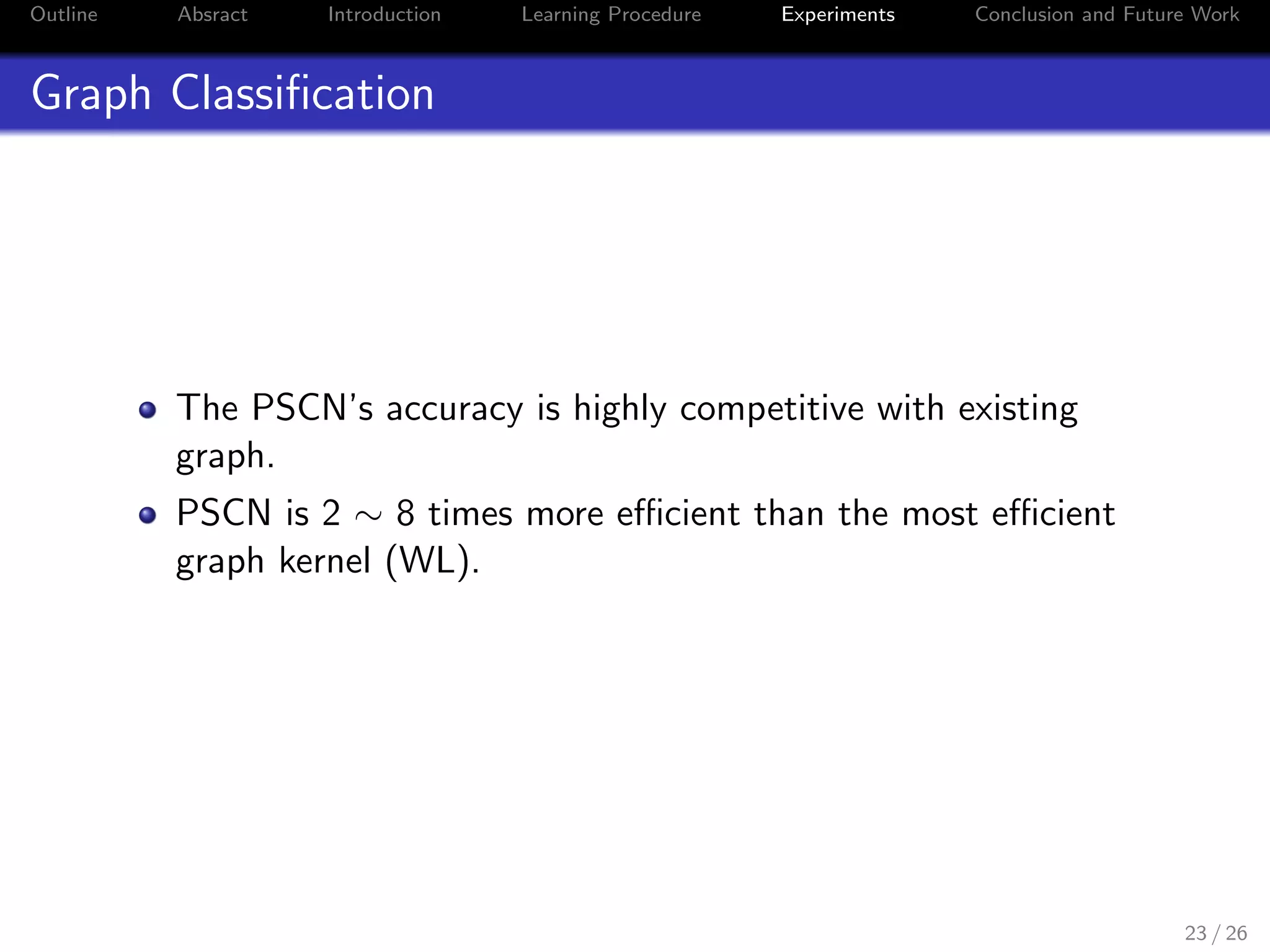
Graph Classification
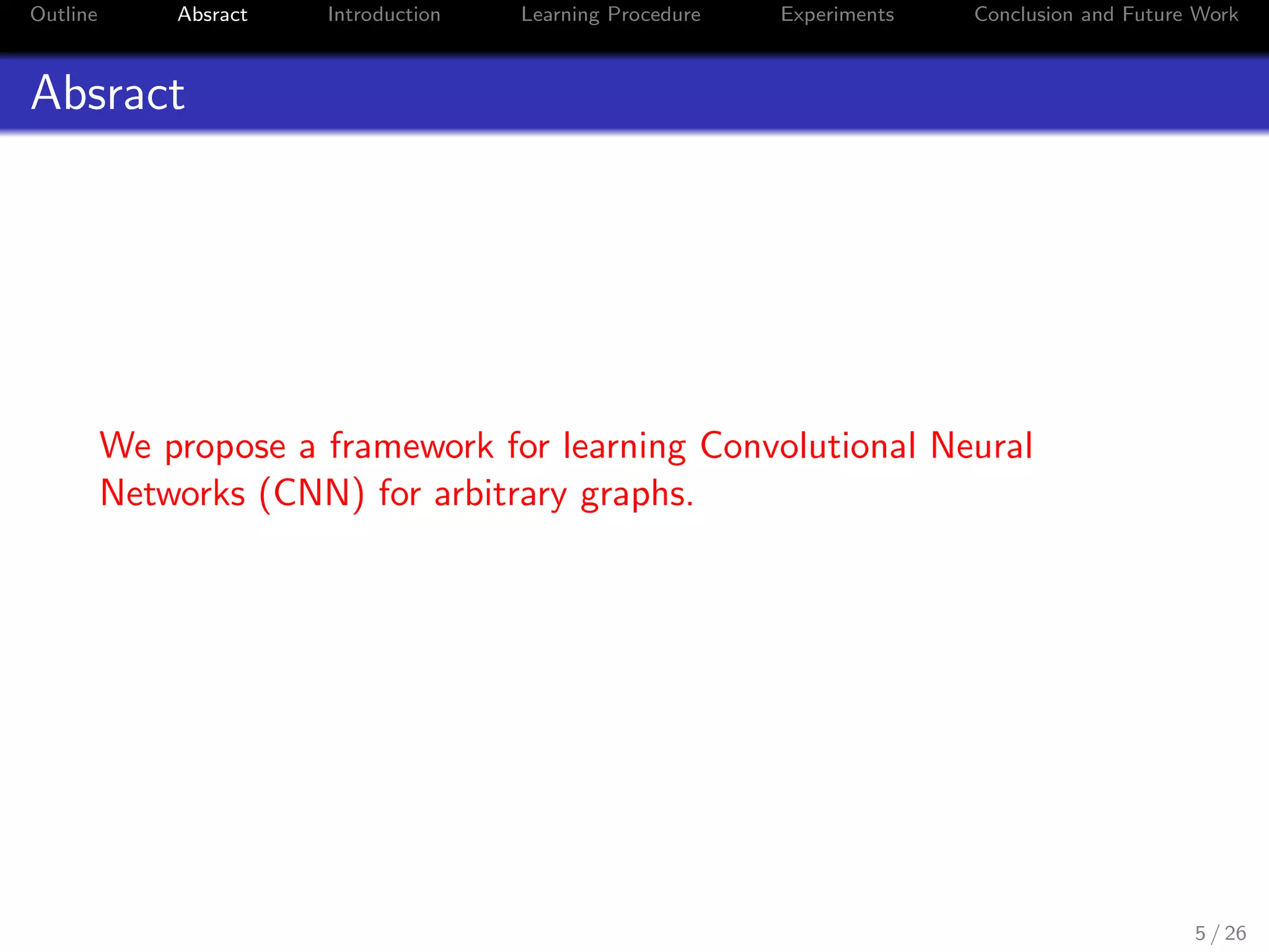
Learning Convolutional Neural Networks for Graphs
Data set MUTAG PCT NCI1 PROTEIN D & D
Max 28 109 111 620 5748
Avg 17.93 25.56 29.87 39.06 284.32
Graphs 188 344 4110 1113 1178
SP [7] 85.79 ± 2.51 58.53 ± 2.55 73.00 ± 0.51 75.07 ± 0.54 > 3 days
RW [17] 83.68 ± 1.66 57.26 ± 1.30 > 3 days 74.22 ± 0.42 > 3 days
GK [38] 81.58 ± 2.11 57.32 ± 1.13 62.28 ± 0.29 71.67 ± 0.55 78.45 ± 0.26
WL [39] 80.72 ± 3.00 (5s) 56.97 ± 2.01 (30s) 80.22 ± 0.51 (375s) 72.92 ± 0.56 (143s) 77.95 ± 0.70 (609s)
PSCN k=5 91.58 ± 5.86 (2s) 59.43 ± 3.14 (4s) 72.80 ± 2.06 (59s) 74.10 ± 1.72 (22s) 74.58 ± 2.85 (121s)
PSCN k=10 88.95 ± 4.37 (3s) 62.29 ± 5.68 (6s) 76.34 ± 1.68 (76s) 75.00 ± 2.51 (30s) 76.27 ± 2.64 (154s)
PSCN k=10E
92.63 ± 4.21 (3s) 60.00 ± 4.82 (6s) 78.59 ± 1.89 (76s) 75.89 ± 2.76 (30s) 77.12 ± 2.41 (154s)
PSLR k=10 87.37 ± 7.88 58.57 ± 5.46 70.00 ± 1.98 71.79 ± 3.71 68.39 ± 5.56
Table 1. Properties of the data sets and accuracy and timing results (in seconds) for PATCHY-SAN and 4 state of the art graph kernels.
Data set GK [38] DGK [45] PSCN k=10
COLLAB 72.84 ± 0.28 73.09 ± 0.25 72.60 ± 2.15
IMDB-B 65.87 ± 0.98 66.96 ± 0.56 71.00 ± 2.29
IMDB-M 43.89 ± 0.38 44.55 ± 0.52 45.23 ± 2.84
RE-B 77.34 ± 0.18 78.04 ± 0.39 86.30 ± 1.58
RE-M5k 41.01 ± 0.17 41.27 ± 0.18 49.10 ± 0.70
RE-M10k 31.82 ± 0.08 32.22 ± 0.10 41.32 ± 0.42
Table 2. Comparison of accuracy results on social graphs [45].
parison, we used a single network architecture with two
kernels. In most cases, a receptive field size of 10 results
in the best classification accuracy. The relatively high vari-
ance can be explained with the small size of the bench-
mark data sets and the fact that the CNNs hyperparame-
ters (with the exception of epochs and batch size) were not
tuned to individual data sets. Similar to the experience on
image and text data, we expect PATCHY-SAN to perform
even better for large data sets. Moreover, PATCHY-SAN is
between 2 and 8 times more efficient than the most effi-
cient graph kernel (WL). We expect the performance ad-
vantage to be much more pronounced for data sets with a
Figure 6: Properties of the data sets and accuracy and timing results (in
seconds) where k is the size of the field.
22 / 26

25. Outline Absract Introduction Learning Procedure Experiments Conclusion and Future Work
Graph Classification
The PSCN’s accuracy is highly competitive with existing
graph.
PSCN is 2 ∼ 8 times more efficient than the most efficient
graph kernel (WL).
23 / 26

26. Outline Absract Introduction Learning Procedure Experiments Conclusion and Future Work
1 Absract
2 Introduction
3 Learning Procedure
4 Experiments
5 Conclusion and Future Work
24 / 26

27. Outline Absract Introduction Learning Procedure Experiments Conclusion and Future Work
Conclusion
We proposed a framework for learning graph
representations that are especially beneficial in
conjunction with CNNs.
Procedure
1 select a sequence of nodes
2 generate local normalized neighborhood representations for
each of the nodes in the sequence
25 / 26

28. Outline Absract Introduction Learning Procedure Experiments Conclusion and Future Work
Future Work
RNNs
different receptive field sizes
pretraining with RBMs and autoencoders
statistical relational models
26 / 26