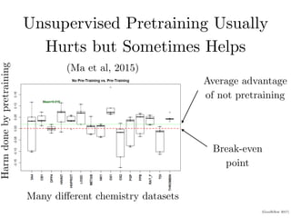
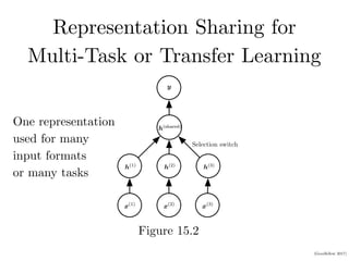
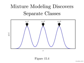
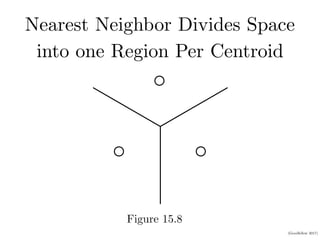
1. Unsupervised pretraining of deep neural networks (DNNs) on multiple datasets usually provides no benefit and sometimes harms performance compared to DNNs trained on individual datasets. 2. Representation learning aims to learn representations of input data that make a task easier by separating explanatory factors of variations. For example, mixture models can discover separate classes in data and distributed representations can divide the input space into uniquely identifiable regions. 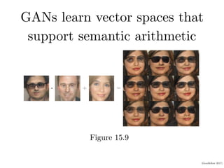3. Generative adversarial networks (GANs) can learn vector spaces that support semantic operations like representing a woman with glasses by combining vectors for concepts of gender and wearing glasses.

1. Representation
Learning
Lecture slides for Chapter 15 of Deep Learning
www.deeplearningbook.org
Ian Goodfellow
2017-10-03

2. (Goodfellow 2017)
Unsupervised Pretraining Usually
Hurts but Sometimes Helps
een joint DNNs trained with multiple data sets and the individual DNNs trained with single data sets. Each column
omparing joint DNNs with single-task DNNs. Each circle represents the difference, measured in R2
, of a pair of DNNs
sets and a single data set, respectively. The horizontal dashed red line indicates 0. A positive value indicates the case where
an individual DNN. The p-value of a two-side paired-sample t test conducted for each scenario is also provided at the
ervised pretraining. Each column represents a QSAR data set, and each circle represents the difference, measured in R2
, of
hout and with pretraining, respectively. The horizontal dashed red line indicates 0. A positive value indicates that a DNN
performs the corresponding DNN with a pretraining. The horizontal dotted green line indicates the overall difference
nd with pretraining, measured in mean R2
.
(Ma et al, 2015)
Break-even
point
Average advantage
of not pretraining
Harm
done
by
pretraining
Many different chemistry datasets

3. (Goodfellow 2017)
Pretraining Changes Learning
Trajectory
−4000 −3000 −2000 −1000 0 1000 2000 3000 4000
−1500
−1000
−500
0
500
1000
1500
With pretraining
Without pretraining
ure 15.1: Visualization via nonlinear projection of the learning trajectories of di
ral networks in function space (not parameter space, to avoid the issue of many-
Figure 15.1

4. (Goodfellow 2017)
Representation Sharing for
Multi-Task or Transfer Learning
CHAPTER 15. REPRESENTATION LEARNING
Selection switch
h(1)
h(1)
h(2)
h(2)
h(3)
h(3)
y
y
h(shared)
h(shared)
x(1)
x(1)
x(2)
x(2)
x(3)
x(3)
Figure 15.2: Example architecture for multitask or transfer learning when the output
variable y has the same semantics for all tasks while the input variable x has a different
Figure 15.2
One representation
used for many
input formats
or many tasks

5. (Goodfellow 2017)
Zero Shot Learning
CHAPTER 15. REPRESENTATION LEARNING
hx = fx(x)
xtest
ytest
hy = fy(y)
y space
Relationship between embedded points within one of the domains
Maps between representation spaces
fx
fy
x space
(x, y) pairs in the training set
fx : encoder function for x
fy : encoder function for y
Figure 15.3: Transfer learning between two domains x and y enables zero-shot learning.
Labeled or unlabeled examples of x allow one to learn a representation function fx and
similarly with examples of y to learn f . Each application of the f and f functions
Figure 15.3

6. (Goodfellow 2017)
Mixture Modeling Discovers
Separate Classes
HAPTER 15. REPRESENTATION LEARNING
x
p(x)
y=1 y=2 y=3
gure 15.4: Mixture model. Example of a density over x that is a mixture over thre
mponents. The component identity is an underlying explanatory factor, y. Because th
Figure 15.4

7. (Goodfellow 2017)
Mean Squared Error Can Ignore
Small but Task-Relevant Features
Figure 15.5
CHAPTER 15. REPRESENTATION LEARNING
Input Reconstruction
Figure 15.5: An autoencoder trained with mean squared error for a robotics task has
failed to reconstruct a ping pong ball. The existence of the ping pong ball and all its
spatial coordinates are important underlying causal factors that generate the image and
are relevant to the robotics task. Unfortunately, the autoencoder has limited capacity,
and the training with mean squared error did not identify the ping pong ball as being
salient enough to encode. Images graciously provided by Chelsea Finn.
The ping pong ball vanishes because it is not large
enough to significantly affect the mean squared error

8. (Goodfellow 2017)
Adversarial Losses Preserve Any Features
with Highly Structured Patterns
Figure 15.6
CHAPTER 15. REPRESENTATION LEARNING
Ground Truth MSE Adversarial
Figure 15.6: Predictive generative networks provide an example of the importance of
learning which features are salient. In this example, the predictive generative network
has been trained to predict the appearance of a 3-D model of a human head at a specific
viewing angle. (Left)Ground truth. This is the correct image, which the network should
emit. (Center)Image produced by a predictive generative network trained with mean
squared error alone. Because the ears do not cause an extreme difference in brightness
compared to the neighboring skin, they were not sufficiently salient for the model to learn
Mean squared error loses the ear because it causes a
small change in few pixels. Adversarial loss preserves
the ear because it is easy to notice its absence.

9. (Goodfellow 2017)
Binary Distributed Representations Divide
Space Into Many Uniquely Identifiable Regions
CHAPTER 15. REPRESENTATION LEARNING
h1
h2 h3
h = [1, 1, 1]>
h = [0, 1, 1]>
h = [1, 0, 1]>
h = [1, 1, 0]>
h = [0, 1, 0]>
h = [0, 0, 1]>
h = [1, 0, 0]>
Figure 15.7: Illustration of how a learning algorithm based on a distributed representation
breaks up the input space into regions. In this example, there are three binary features
h1, h2, and h3. Each feature is defined by thresholding the output of a learned linear
Figure 15.7

10. (Goodfellow 2017)
Binary Distributed Representations Divide
Space Into Many Uniquely Identifiable Regions
CHAPTER 15. REPRESENTATION LEARNING
h1
h2 h3
h = [1, 1, 1]>
h = [0, 1, 1]>
h = [1, 0, 1]>
h = [1, 1, 0]>
h = [0, 1, 0]>
h = [0, 0, 1]>
h = [1, 0, 0]>
Figure 15.7: Illustration of how a learning algorithm based on a distributed representation
breaks up the input space into regions. In this example, there are three binary features
h1, h2, and h3. Each feature is defined by thresholding the output of a learned linear
Figure 15.7

11. (Goodfellow 2017)
Nearest Neighbor Divides Space
into one Region Per Centroid
e 15.8: Illustration of how the nearest neighbor algorithm breaks up the input
different regions. The nearest neighbor algorithm provides an example of a lea
Figure 15.8

12. (Goodfellow 2017)
GANs learn vector spaces that
support semantic arithmetic
CHAPTER 15. REPRESENTATION LEARNING
- + =
Figure 15.9: A generative model has learned a distributed representation that disentangles
the concept of gender from the concept of wearing glasses. If we begin with the repre-
sentation of the concept of a man with glasses, then subtract the vector representing the
concept of a man without glasses, and finally add the vector representing the concept
of a woman without glasses, we obtain the vector representing the concept of a woman
Figure 15.9