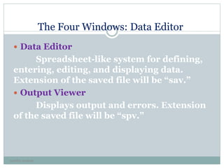
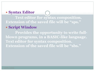
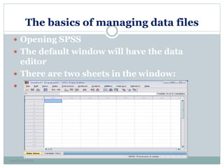
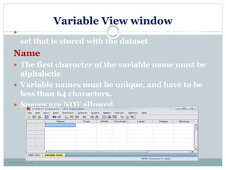
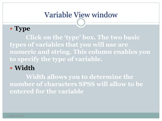
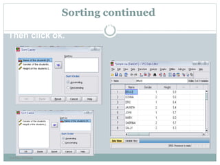
neethu asokan
 The software name stands for Statistical
Package for the Social Sciences (SPSS)
 Reflecting the original market, although the
software is now popular in other fields as
well, including the health sciences and
marketing.
 Used to analyze data collected from surveys,
tests, observations, etc. It can perform a
variety of data analyses and presentation
functions, including statistical analysis and
graphical presentation of data.
neethu asokan
Statistics included in the base
software:
 Descriptive statistics: Cross tabulation,
Frequencies, Descriptives, Explore,
Descriptive Ratio Statistics
 Bivariate statistics: Means, t-test,
ANOVA, Correlation (bivariate, partial,
distances), Nonparametric tests
 Prediction for numerical outcomes:
Linear regression
 Prediction for identifying groups: Factor
analysis, cluster analysis (two-step, K-
means, hierarchical), Discriminant
neethu asokan
History
 The software was released in its first version
in 1968 as the Statistical Package for the
Social Sciences (SPSS) after being developed
by Norman H. Nie, Dale H. Bent, and C.
Hadlai Hull
 Those principals incorporated as SPSS Inc.
in 1975
neethu asokan
Objectives
 About the four-windows in SPSS
 The basics of managing data files
 The basic analysis in SPSS
neethu asokan
The Four Windows: Data Editor
 Data Editor
Spreadsheet-like system for defining,
entering, editing, and displaying data.
Extension of the saved file will be “sav.”
 Output Viewer
Displays output and errors. Extension
of the saved file will be “spv.”
neethu asokan
 Syntax Editor
Text editor for syntax composition.
Extension of the saved file will be “sps.”
 Script Window
Provides the opportunity to write full-
blown programs, in a BASIC-like language.
Text editor for syntax composition.
Extension of the saved file will be “sbs.”
neethu asokan
The basics of managing data files
 Opening SPSS
 The default window will have the data
editor
 There are two sheets in the window:
 1. Data view 2. Variable view
neethu asokan
Data View window
The Data View window
 This sheet is visible when you first open the Data
Editor and this sheet contains the data
 Click on the tab labeled Variable View
neethu asokan
Variable View window
 This sheet contains information about the data
set that is stored with the dataset
Name
 The first character of the variable name must be
alphabetic
 Variable names must be unique, and have to be
less than 64 characters.
 Spaces are NOT allowed.
neethu asokan
Variable View window
 Type
Click on the ‘type’ box. The two basic
types of variables that you will use are
numeric and string. This column enables you
to specify the type of variable.
 Width
Width allows you to determine the
number of characters SPSS will allow to be
entered for the variable
neethu asokan
 Decimals
Number of decimals
It has to be less than or equal to 16
 Label
You can specify the details of the variable
You can write characters with spaces up to 256
characters
 Values
This is used and to suggest which numbers
represent which categories when the variable
represents a category
neethu asokan
Defining the value labels
 Click the cell in the values column as shown below
 For the value, and the label, you can put up to 60
characters.
 After defining the values click add and then click OK.
neethu asokan
Example
neethu asokan
Example (solution)
neethu asokan
neethu asokan
Sorting the data
neethu asokan
Sorting continued
Double Click ‘Name of the students.’
Then click ok.
neethu asokan
References
 Kentaka Aruga (Feb 2008), Introduction To SPSS
(pdf).
 SPSS wikepedia, the free encyclopedia.
 SPSS_brief guide_21.pdf
 SPSS_ statistics_17.pdf
neethu asokan
Response Surface Methodology
neethu asokan
Definition of Response Surface Method
A simple function, such as linear or quadratic
polynomial, fitted to the data obtained from the
experiments is called a response surface, and the
approach is called the response surface method.
Response surface method is a collection of
statistical and mathematical techniques useful for
developing, improving, and optimizing processes.
Response surface method is a method for
constructing global approximations to system
behavior based on results calculated at various
points in the design space.
Box G.E.P. and Draper N.R.,1987
Myers R.H., 1995
Roux W.J.,1998
neethu asokan
RSM
 Response surface methodology (RSM) is a useful statistical
technique which has been applied in research into complex
variation process.
 The multiple regression and correlation analyses are used as
tools to assess the effects of two or more independent factors
on the dependent variable.
 Further more, the central composite design (CCD) of RSM has
been applied in the optimization of several biotechnological
and chemical processes (Jeong et al., 2009).
 Its main advantage is the reduced number of experimental runs
required to generate sufficient information for a statistically
acceptable results.
neethu asokan
History of Response Surface Method
1951 Box and Wilson - CCD
1959 Kiefer - Start of D-optimal Design
1960 Box and Behnken - Box-Behnken deign
1971 Box and Draper - D-optimal Design
1972 Fedorov - exchange algorithm
1974 Mitchell - D-optimal Design
1996 Burgee - design HSCT
1997 Ragon and Haftka - optimization of large wing structure
1998 Koch, Mavris, and Mistree - multi-level approximation
1999 Choi / Mavris – Robut, Reliablity-Based Design
Research of DOE
Application in
Optimization
App in Optimization & Reduce the
Approximation Error
neethu asokan
Concept of Response Surface Method
Original System
x1
x
2
-1 0 1
1
0
-1
DOE and Experiments
Black Boxed
System
Input
1x
2x
Response
y
RS Model
  jiiiiiiii xxbxbxbby
2
0
neethu asokan
Designs
 Three level factorial
 Box- Behnken
 Central Composite Design
 Doeblert designs
 Plackett- Burman JMP
In-
House
c
odes
Visual-
DOC SAS
SPS
S
MATLAB
Softwares
neethu asokan
Example
 Optimization of clavulanic acid production by Streptomyces
DAUFPE 3060 by response surface methodology.
 Clavulanic acid (CA) is a β-lactamase inhibitor that is
administered in combination with penicillin group antibiotics to
overcome certain types of antibiotic resistance.
 In order to optimize its production by the new isolate
Streptomyces DAUFPE 3060, the influence of two independent
variables, temperature and soybean flour concentration, on
clavulanic acid and biomass concentrations was investigated in
250 mL-Erlenmeyers according to central composite designs.
neethu asokan
Contin….
 A central composite design combined with RSM was used in
this work to select the best values of these two variables able to
optimize CA production by the same strain.
Method
Fermentation Spores
Liquid media/96h
Initial biomass concentration
Spores are stored by lyophilized in glycerol 10% v/v
Seed culture
neethu asokan
Cryotube with glycerol to 25ml of seed medium in 250ml flask
Incubated under shaker (28ºc, 200rpm, 24hrs.)
45ml of inoculum inoculated with 5ml of seed culture in 250ml flask
14 production runs, which lasted 168h
(orbital shaker/ 150rpm at different temp).
5ml of aliquots of
this suspension
with cells at
exponential phase
Flask containing
45ml production
media
neethu asokan
Experimental design
 The quadratic model to predict the optimal point was expressed
by the equation:
 where Ŷ represents the predicted value of the response variables,
b0 is the intercept coefficient, bi are the linear coefficients, bii
are the quadratic coefficients and bij are the interaction ones.
neethu asokan
Experimental design
 Experiments were planned so as to obtain quadratic models
able to describe the CA and biomass concentrations as
simultaneous functions of temperature and SF levels.
• The statistical significance of the regression coefficients was
determined by the Student's t-test, and the second-order
model equation was determined by the Fischer's test.
• The effects of unexplained variability in the observed
response due to extraneous factors were minimized by
randomizing the order of experiments
neethu asokan
neethu asokan
Experimental design conti………
 The experimental data of Table 2 were then used to make
regression analyses fitting both responses. The following
equations, where the variables take their coded values, express
the best models for CA and biomass concentrations,
respectively:
 where Ŷ1,Ŷ2 and x1 are CA, biomass and SF concentrations,
while x2 is temperature.
neethu asokan
 The simultaneous effects
of temperature and SF
concentration and their
interactions on the CA and
biomass productions are
better visualized in three-
dimensional (3-D) graph
projections (Figures 1 and
2) using the Response
Surface Methodology
(RSM).
Figure 1
neethu asokan
This means that the values
of both responses increased
up to a certain level when
both variables were raised.
As a result, there are two
regions of temperature (30-
34°C) and SF concentration
(35-45 g/L) where both
responses reach maximum
values.
Figure 2
neethu asokan
RESULT
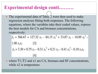
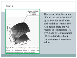
 Simultaneous regression by eqs. [3] and [4] provided maximum
predicted values of CA concentration (640 mg/L) at 33.0 °C and
SF = 37.5 g/L, and of biomass concentration (3.75 g/L) at 30.2 °C
and SF = 41.77 g/L, respectively. These predicted values are only
1.7 % higher and 3.8% lower than the experimental ones, thus
demonstrating the validity of the models employed.
neethu asokan
 Heavy Computation Problem
Approximation
 When Sensitivity is NOT Available
 Real / Numerical Experiment
 When the Batch Run is Impossible
 For Any System Which has Inputs
and Responses
 Easy to Implement
 Probabilistic Concept
 Noisy Responses or Environments
• Approximation Error
• Domain is Very Dominant
Advantages
Disadvantages
neethu asokan
Conclusion
 Response surface methods (RSM) provide
statistically-validated predictive models that can
then be manipulated for finding optimal process
configurations.
 The optimum conditions for clavulanic acid
production were determined with the aid of the
central composite design (CCD).
neethu asokan
References
 Daniela A. et.al., Optimization of clavulanic acid production by
Streptomyces DAUFPE 3060 by response surface methodology,
Braz. J. Microbiol. vol.42 no.2 São Paulo Apr./June 2011.
 Nadeem Irfan Bukhari et. Al.,Statistical Design of Experiments
on Fabrication of Starch Nanoparticles – A Case Study for
Application of Response Surface Methods (RSM).
 Response surface methodology,ppt.
 Tanarkorn Sukjit1& Vittaya Punsuvon1,Process Optimization Of
Crude Palm Oil Biodiesel Production By Response Surface
methodology, European International Journal of Science and
Technology Vol. 2 No. 7 September 2013.
neethu asokan
Thank
you
neethu asokan

Spss & rsm copy

  • 1.
  • 2.
     The softwarename stands for Statistical Package for the Social Sciences (SPSS)  Reflecting the original market, although the software is now popular in other fields as well, including the health sciences and marketing.  Used to analyze data collected from surveys, tests, observations, etc. It can perform a variety of data analyses and presentation functions, including statistical analysis and graphical presentation of data. neethu asokan
  • 3.
    Statistics included inthe base software:  Descriptive statistics: Cross tabulation, Frequencies, Descriptives, Explore, Descriptive Ratio Statistics  Bivariate statistics: Means, t-test, ANOVA, Correlation (bivariate, partial, distances), Nonparametric tests  Prediction for numerical outcomes: Linear regression  Prediction for identifying groups: Factor analysis, cluster analysis (two-step, K- means, hierarchical), Discriminant neethu asokan
  • 4.
    History  The softwarewas released in its first version in 1968 as the Statistical Package for the Social Sciences (SPSS) after being developed by Norman H. Nie, Dale H. Bent, and C. Hadlai Hull  Those principals incorporated as SPSS Inc. in 1975 neethu asokan
  • 5.
    Objectives  About thefour-windows in SPSS  The basics of managing data files  The basic analysis in SPSS neethu asokan
  • 6.
    The Four Windows:Data Editor  Data Editor Spreadsheet-like system for defining, entering, editing, and displaying data. Extension of the saved file will be “sav.”  Output Viewer Displays output and errors. Extension of the saved file will be “spv.” neethu asokan
  • 7.
     Syntax Editor Texteditor for syntax composition. Extension of the saved file will be “sps.”  Script Window Provides the opportunity to write full- blown programs, in a BASIC-like language. Text editor for syntax composition. Extension of the saved file will be “sbs.” neethu asokan
  • 8.
    The basics ofmanaging data files  Opening SPSS  The default window will have the data editor  There are two sheets in the window:  1. Data view 2. Variable view neethu asokan
  • 9.
    Data View window TheData View window  This sheet is visible when you first open the Data Editor and this sheet contains the data  Click on the tab labeled Variable View neethu asokan
  • 10.
    Variable View window This sheet contains information about the data set that is stored with the dataset Name  The first character of the variable name must be alphabetic  Variable names must be unique, and have to be less than 64 characters.  Spaces are NOT allowed. neethu asokan
  • 11.
    Variable View window Type Click on the ‘type’ box. The two basic types of variables that you will use are numeric and string. This column enables you to specify the type of variable.  Width Width allows you to determine the number of characters SPSS will allow to be entered for the variable neethu asokan
  • 12.
     Decimals Number ofdecimals It has to be less than or equal to 16  Label You can specify the details of the variable You can write characters with spaces up to 256 characters  Values This is used and to suggest which numbers represent which categories when the variable represents a category neethu asokan
  • 13.
    Defining the valuelabels  Click the cell in the values column as shown below  For the value, and the label, you can put up to 60 characters.  After defining the values click add and then click OK. neethu asokan
  • 14.
  • 15.
  • 16.
  • 17.
  • 18.
    Sorting continued Double Click‘Name of the students.’ Then click ok. neethu asokan
  • 19.
    References  Kentaka Aruga(Feb 2008), Introduction To SPSS (pdf).  SPSS wikepedia, the free encyclopedia.  SPSS_brief guide_21.pdf  SPSS_ statistics_17.pdf neethu asokan
  • 20.
  • 21.
    Definition of ResponseSurface Method A simple function, such as linear or quadratic polynomial, fitted to the data obtained from the experiments is called a response surface, and the approach is called the response surface method. Response surface method is a collection of statistical and mathematical techniques useful for developing, improving, and optimizing processes. Response surface method is a method for constructing global approximations to system behavior based on results calculated at various points in the design space. Box G.E.P. and Draper N.R.,1987 Myers R.H., 1995 Roux W.J.,1998 neethu asokan
  • 22.
    RSM  Response surfacemethodology (RSM) is a useful statistical technique which has been applied in research into complex variation process.  The multiple regression and correlation analyses are used as tools to assess the effects of two or more independent factors on the dependent variable.  Further more, the central composite design (CCD) of RSM has been applied in the optimization of several biotechnological and chemical processes (Jeong et al., 2009).  Its main advantage is the reduced number of experimental runs required to generate sufficient information for a statistically acceptable results. neethu asokan
  • 23.
    History of ResponseSurface Method 1951 Box and Wilson - CCD 1959 Kiefer - Start of D-optimal Design 1960 Box and Behnken - Box-Behnken deign 1971 Box and Draper - D-optimal Design 1972 Fedorov - exchange algorithm 1974 Mitchell - D-optimal Design 1996 Burgee - design HSCT 1997 Ragon and Haftka - optimization of large wing structure 1998 Koch, Mavris, and Mistree - multi-level approximation 1999 Choi / Mavris – Robut, Reliablity-Based Design Research of DOE Application in Optimization App in Optimization & Reduce the Approximation Error neethu asokan
  • 24.
    Concept of ResponseSurface Method Original System x1 x 2 -1 0 1 1 0 -1 DOE and Experiments Black Boxed System Input 1x 2x Response y RS Model   jiiiiiiii xxbxbxbby 2 0 neethu asokan
  • 25.
    Designs  Three levelfactorial  Box- Behnken  Central Composite Design  Doeblert designs  Plackett- Burman JMP In- House c odes Visual- DOC SAS SPS S MATLAB Softwares neethu asokan
  • 26.
    Example  Optimization ofclavulanic acid production by Streptomyces DAUFPE 3060 by response surface methodology.  Clavulanic acid (CA) is a β-lactamase inhibitor that is administered in combination with penicillin group antibiotics to overcome certain types of antibiotic resistance.  In order to optimize its production by the new isolate Streptomyces DAUFPE 3060, the influence of two independent variables, temperature and soybean flour concentration, on clavulanic acid and biomass concentrations was investigated in 250 mL-Erlenmeyers according to central composite designs. neethu asokan
  • 27.
    Contin….  A centralcomposite design combined with RSM was used in this work to select the best values of these two variables able to optimize CA production by the same strain. Method Fermentation Spores Liquid media/96h Initial biomass concentration Spores are stored by lyophilized in glycerol 10% v/v Seed culture neethu asokan
  • 28.
    Cryotube with glycerolto 25ml of seed medium in 250ml flask Incubated under shaker (28ºc, 200rpm, 24hrs.) 45ml of inoculum inoculated with 5ml of seed culture in 250ml flask 14 production runs, which lasted 168h (orbital shaker/ 150rpm at different temp). 5ml of aliquots of this suspension with cells at exponential phase Flask containing 45ml production media neethu asokan
  • 29.
    Experimental design  Thequadratic model to predict the optimal point was expressed by the equation:  where Ŷ represents the predicted value of the response variables, b0 is the intercept coefficient, bi are the linear coefficients, bii are the quadratic coefficients and bij are the interaction ones. neethu asokan
  • 30.
    Experimental design  Experimentswere planned so as to obtain quadratic models able to describe the CA and biomass concentrations as simultaneous functions of temperature and SF levels. • The statistical significance of the regression coefficients was determined by the Student's t-test, and the second-order model equation was determined by the Fischer's test. • The effects of unexplained variability in the observed response due to extraneous factors were minimized by randomizing the order of experiments neethu asokan
  • 31.
  • 32.
    Experimental design conti……… The experimental data of Table 2 were then used to make regression analyses fitting both responses. The following equations, where the variables take their coded values, express the best models for CA and biomass concentrations, respectively:  where Ŷ1,Ŷ2 and x1 are CA, biomass and SF concentrations, while x2 is temperature. neethu asokan
  • 33.
     The simultaneouseffects of temperature and SF concentration and their interactions on the CA and biomass productions are better visualized in three- dimensional (3-D) graph projections (Figures 1 and 2) using the Response Surface Methodology (RSM). Figure 1 neethu asokan
  • 34.
    This means thatthe values of both responses increased up to a certain level when both variables were raised. As a result, there are two regions of temperature (30- 34°C) and SF concentration (35-45 g/L) where both responses reach maximum values. Figure 2 neethu asokan
  • 35.
    RESULT  Simultaneous regressionby eqs. [3] and [4] provided maximum predicted values of CA concentration (640 mg/L) at 33.0 °C and SF = 37.5 g/L, and of biomass concentration (3.75 g/L) at 30.2 °C and SF = 41.77 g/L, respectively. These predicted values are only 1.7 % higher and 3.8% lower than the experimental ones, thus demonstrating the validity of the models employed. neethu asokan
  • 36.
     Heavy ComputationProblem Approximation  When Sensitivity is NOT Available  Real / Numerical Experiment  When the Batch Run is Impossible  For Any System Which has Inputs and Responses  Easy to Implement  Probabilistic Concept  Noisy Responses or Environments • Approximation Error • Domain is Very Dominant Advantages Disadvantages neethu asokan
  • 37.
    Conclusion  Response surfacemethods (RSM) provide statistically-validated predictive models that can then be manipulated for finding optimal process configurations.  The optimum conditions for clavulanic acid production were determined with the aid of the central composite design (CCD). neethu asokan
  • 38.
    References  Daniela A.et.al., Optimization of clavulanic acid production by Streptomyces DAUFPE 3060 by response surface methodology, Braz. J. Microbiol. vol.42 no.2 São Paulo Apr./June 2011.  Nadeem Irfan Bukhari et. Al.,Statistical Design of Experiments on Fabrication of Starch Nanoparticles – A Case Study for Application of Response Surface Methods (RSM).  Response surface methodology,ppt.  Tanarkorn Sukjit1& Vittaya Punsuvon1,Process Optimization Of Crude Palm Oil Biodiesel Production By Response Surface methodology, European International Journal of Science and Technology Vol. 2 No. 7 September 2013. neethu asokan
  • 39.