MTH 201: Biometry
Lecture Notes
October 2013
2
Department of Biometry and Mathematics
Faculty of Science
Sokoine University of Agriculture
MTH 201: Biometry
Lecture Notes
Kassile, T.
Office Room # 9, KEPA, SMC, Mazimbu
Table of Contents
Preface . . . . . . . . . . . . . . . . . . . . . . . . . . . . . . . . . . . . . v
0.1 Preface . . . . . . . . . . . . . . . . . . . . . . . . . . . . . . . . . . v
0.1.1 Course Objective . . . . . . . . . . . . . . . . . . . . . . . . . v
0.1.2 Course Description . . . . . . . . . . . . . . . . . . . . . . . . v
0.1.3 Pre-requisite . . . . . . . . . . . . . . . . . . . . . . . . . . . v
0.1.4 Course requirement . . . . . . . . . . . . . . . . . . . . . . . v
0.1.5 Computing . . . . . . . . . . . . . . . . . . . . . . . . . . . . v
0.1.6 References . . . . . . . . . . . . . . . . . . . . . . . . . . . . . v
1 Terminologies in Experimental Designs 1
1.1 Introduction . . . . . . . . . . . . . . . . . . . . . . . . . . . . . . . . 1
1.1.1 Definitions . . . . . . . . . . . . . . . . . . . . . . . . . . . . 1
2 Principles of experimental designs 5
2.1 Introduction . . . . . . . . . . . . . . . . . . . . . . . . . . . . . . . . 5
2.2 Randomization principle . . . . . . . . . . . . . . . . . . . . . . . . . 5
2.3 Replication principle . . . . . . . . . . . . . . . . . . . . . . . . . . . 6
2.4 Local control principle . . . . . . . . . . . . . . . . . . . . . . . . . . 7
3 Analysis of Variance 9
3.1 Introduction . . . . . . . . . . . . . . . . . . . . . . . . . . . . . . . . 9
3.2 Assumptions in the analysis of variance . . . . . . . . . . . . . . . . 10
3.3 Analysis of variance for one-way classification . . . . . . . . . . . . . 11
3.3.1 Analysis of variance for one-way classification with unequal
replication (unbalanced data) . . . . . . . . . . . . . . . . . . 11
3.3.2 Linear additive model for one-way classification . . . . . . . . 12
3.3.3 Fixed vs. random effects . . . . . . . . . . . . . . . . . . . . . 12
i
ii TABLE OF CONTENTS
3.3.4 Calculation of sums of squares . . . . . . . . . . . . . . . . . 13
3.3.5 ANOVA for one-way classification with equal replication (bal-
anced data) . . . . . . . . . . . . . . . . . . . . . . . . . . . . 19
3.4 ANOVA for two-way classification (Without Replication) . . . . . . 21
3.4.1 Linear additive model for two-way classification . . . . . . . . 21
3.5 The least significance difference (LSD) . . . . . . . . . . . . . . . . . 25
4 Introduction to SPSS 29
4.1 Introduction . . . . . . . . . . . . . . . . . . . . . . . . . . . . . . . . 29
4.2 Starting SPSS . . . . . . . . . . . . . . . . . . . . . . . . . . . . . . . 30
4.3 Data entry . . . . . . . . . . . . . . . . . . . . . . . . . . . . . . . . 32
4.4 Keying data into SPSS . . . . . . . . . . . . . . . . . . . . . . . . . . 32
4.4.1 Osteopathic manipulation data set . . . . . . . . . . . . . . . 32
4.5 Opening an existing dataset . . . . . . . . . . . . . . . . . . . . . . . 34
4.6 Importing data . . . . . . . . . . . . . . . . . . . . . . . . . . . . . . 35
4.7 Exporting data . . . . . . . . . . . . . . . . . . . . . . . . . . . . . . 35
4.8 ANOVA for one-way classification in SPSS . . . . . . . . . . . . . . . 35
5 Completely Randomized Design 39
5.1 Introduction . . . . . . . . . . . . . . . . . . . . . . . . . . . . . . . . 39
5.2 Layout . . . . . . . . . . . . . . . . . . . . . . . . . . . . . . . . . . . 39
5.3 Statistical analysis . . . . . . . . . . . . . . . . . . . . . . . . . . . . 40
5.3.1 Statistical hypotheses . . . . . . . . . . . . . . . . . . . . . . 40
5.3.2 Test procedure . . . . . . . . . . . . . . . . . . . . . . . . . . 41
5.4 Advantages and disadvantages of CRD . . . . . . . . . . . . . . . . . 41
5.4.1 Advantages . . . . . . . . . . . . . . . . . . . . . . . . . . . . 41
5.4.2 Disadvantages . . . . . . . . . . . . . . . . . . . . . . . . . . . 41
5.5 Example . . . . . . . . . . . . . . . . . . . . . . . . . . . . . . . . . . 41
6 Randomised Block Design 45
6.1 Introduction . . . . . . . . . . . . . . . . . . . . . . . . . . . . . . . . 45
6.2 Layout . . . . . . . . . . . . . . . . . . . . . . . . . . . . . . . . . . . 46
6.3 Statistical analysis . . . . . . . . . . . . . . . . . . . . . . . . . . . . 47
6.3.1 Statistical hypotheses . . . . . . . . . . . . . . . . . . . . . . 47
6.3.2 Test procedure . . . . . . . . . . . . . . . . . . . . . . . . . . 47
TABLE OF CONTENTS iii
6.4 Advantages and disadvantages of RBD . . . . . . . . . . . . . . . . . 48
6.4.1 Advantages . . . . . . . . . . . . . . . . . . . . . . . . . . . . 48
6.4.2 Disadvantages . . . . . . . . . . . . . . . . . . . . . . . . . . . 48
6.5 Example . . . . . . . . . . . . . . . . . . . . . . . . . . . . . . . . . . 48
6.6 Reasons for blocking in RBD . . . . . . . . . . . . . . . . . . . . . . 52
7 Latin Square Design 55
7.1 Introduction . . . . . . . . . . . . . . . . . . . . . . . . . . . . . . . . 55
7.2 Layout . . . . . . . . . . . . . . . . . . . . . . . . . . . . . . . . . . . 55
7.2.1 Linear additive model . . . . . . . . . . . . . . . . . . . . . . 57
7.3 Statistical analysis . . . . . . . . . . . . . . . . . . . . . . . . . . . . 57
7.3.1 Calculation of sums of squares . . . . . . . . . . . . . . . . . 57
7.4 Advantages and disadvantages of LSD . . . . . . . . . . . . . . . . . 58
7.4.1 Advantages . . . . . . . . . . . . . . . . . . . . . . . . . . . . 58
7.4.2 Disadvantages . . . . . . . . . . . . . . . . . . . . . . . . . . . 58
7.5 Example . . . . . . . . . . . . . . . . . . . . . . . . . . . . . . . . . . 59
8 Factorial Experiments 65
8.1 Introduction . . . . . . . . . . . . . . . . . . . . . . . . . . . . . . . . 65
8.2 Main effects and interaction effects . . . . . . . . . . . . . . . . . . . 66
8.3 The 22 factorial experiments . . . . . . . . . . . . . . . . . . . . . . . 66
8.4 The 23 factorial experiments . . . . . . . . . . . . . . . . . . . . . . . 68
8.5 Sum of squares due to factorial effects . . . . . . . . . . . . . . . . . 69
8.6 Tests of significance of factorial effects . . . . . . . . . . . . . . . . . 71
8.7 Yates’ method of computing factorial effect totals . . . . . . . . . . . 74
9 Multiple Comparisons 77
9.1 Introduction . . . . . . . . . . . . . . . . . . . . . . . . . . . . . . . . 77
9.2 Multiple comparisons procedures . . . . . . . . . . . . . . . . . . . . 78
9.2.1 Duncan’s new multiple range-test . . . . . . . . . . . . . . . . 78
10 Simple Linear Regression and Correlation 85
10.1 Simple linear regression . . . . . . . . . . . . . . . . . . . . . . . . . 85
10.1.1 Fitting a simple linear regression model-the method of least
squares . . . . . . . . . . . . . . . . . . . . . . . . . . . . . . 85
iv TABLE OF CONTENTS
10.1.2 Assessing the fitted regression . . . . . . . . . . . . . . . . . . 87
10.1.3 Confidence intervals for regression parameters . . . . . . . . . 93
10.2 Correlation analysis . . . . . . . . . . . . . . . . . . . . . . . . . . . 102
10.2.1 Karl Pearson’s correlation coefficient (r) (ref: MTH 106) . . . 102
10.2.2 Spearman’s coefficient of Rank correlation . . . . . . . . . . . 104
11 Data Transformation 109
11.1 Introduction . . . . . . . . . . . . . . . . . . . . . . . . . . . . . . . . 109
11.2 Parameters of normal distribution . . . . . . . . . . . . . . . . . . . 109
11.2.1 Shape of the normal distribution . . . . . . . . . . . . . . . . 110
11.3 Reasons for data transformation . . . . . . . . . . . . . . . . . . . . 110
11.4 Testing for normality . . . . . . . . . . . . . . . . . . . . . . . . . . . 111
11.5 Common data transformations . . . . . . . . . . . . . . . . . . . . . 111
12 Analysis of Frequency Data 115
12.1 Introduction . . . . . . . . . . . . . . . . . . . . . . . . . . . . . . . . 115
12.2 Objective of two-way classification . . . . . . . . . . . . . . . . . . . 115
12.3 The Chi-square test of independence . . . . . . . . . . . . . . . . . . 117
13 Review Exercises 125
13.1 Exercise I . . . . . . . . . . . . . . . . . . . . . . . . . . . . . . . . . 125
13.2 Exercise II . . . . . . . . . . . . . . . . . . . . . . . . . . . . . . . . . 126
13.3 Exercise III . . . . . . . . . . . . . . . . . . . . . . . . . . . . . . . . 126
13.4 Exercise IV . . . . . . . . . . . . . . . . . . . . . . . . . . . . . . . . 127
13.5 Exercise V . . . . . . . . . . . . . . . . . . . . . . . . . . . . . . . . . 128
13.6 Ecercise VI . . . . . . . . . . . . . . . . . . . . . . . . . . . . . . . . 128
13.7 Exercise VII . . . . . . . . . . . . . . . . . . . . . . . . . . . . . . . . 130
13.8 Exercise VIII . . . . . . . . . . . . . . . . . . . . . . . . . . . . . . . 131
13.9 Exercise IX . . . . . . . . . . . . . . . . . . . . . . . . . . . . . . . . 136
0.1. PREFACE v
0.1 Preface
0.1.1 Course Objective
Focuses on the use of statistical/mathematical techniques to problems in agricul-
tural, environmental, and biological sciences. It is concerned with the design of
experiments, analysis and interpretation of results.
0.1.2 Course Description
Principles of experimental designs, analysis of variance (ANOVA): one way classifica-
tion, e.g., completely randomised design (balanced and unbalanced data), multiway
classification, e.g., randomised complete block design, Latin square design; factorial
experiments. Multiple comparisons, data transformation; simple linear regression
and correlation, analysis of frequency data e.g., contingency tables.
0.1.3 Pre-requisite
MTH 106-Introductory Statistics.
0.1.4 Course requirement
I: Coursework- 2 quizes and 2 tests: contribute 40% of the total credits allotted
to this course.
II: Final (End of Semester) Exam: contribute 60%
0.1.5 Computing
Where necessary, for illustration purposes, the Statistical Package for the Social
Sciences (SPSS) and the SAS software packages will be frequently used. However,
use of SPSS or SAS in the course is considered optional.
0.1.6 References
Cody, R.P. and Smith, J.K. (1997). Applied Statistics and the SAS Programming
Language. Fourth Ed. Prentice Hall.
Der, G. and Everitt, B.S.(2002). A Handbook of Statistical Analyses using SAS.
Second Ed. Chapman & Hall/CRC.
Montgomery, D. (2001). Introduction to Linear Regression Analysis. Wiley and
Sons, Inc.
Montgomery, D. (2001). Design and Analysis of Experiments. Wiley and Sons, Inc.
Neter, J., Kutner, M., Nachetsheim, C. J. and Wasserman, W. (1996). Applied
Linear Statistical Models. Irwin, Chicago.
Chapter 1
Terminologies in Experimental
Designs
1.1 Introduction
Real-life scientific investigations often involve comparisons between several sets of
data collected from basically similar conditions, e.g., groups of plants of the same
type which have been grown under conditions alike except that different fertilizers
were used for each group, different doses of a drug administered to the same or
different groups of patients, different varieties of rations given to a group of homo-
geneous animals, same instructor teaching students with different background about
the subject being taught, etc.
Many types of biological data are collected through planned (well designed) experi-
ments. Designing an experiment requires adherence to some rules or principles and
procedures if valid conclusions are to be drawn. For example, the data from an ex-
periment set up according to a particular design should be analysed according to the
appropriate procedure for that design. No type of statistical method, no matter how
sophisticated, can compensate for a poorly designed study or improve the quality
of results obtained from an improperly designed experiment. Thus, an important
aspect in this respect is that design of experiment determines the quality of the
results! Before we embark on the contents of the course, let us first, briefly distin-
guish between biometry and some related specializations/fields within the statistics
domain.
1.1.1 Definitions
Biometry. As alluded to above, biometry: is a subject that is concerned with the
application of statistics and matehematics to problems in the agricultural, environ-
mental, and biological sciences. Hence, biometrics: is the application of statistics
and mathematics to problems with a biological component, including the problems
in agricultural, environmental, and biological sciences as well as medical science.
1
2 CHAPTER 1. TERMINOLOGIES IN EXPERIMENTAL DESIGNS
These include statistical methods, computational biology, applied mathematics, and
mathematical modeling.
Biostatistics: is a field of study that is concerned with the application of statis-
tics to the biological sciences, especially those relating to medical sciences. Med-
ical colleges/universities (for example, Muhimbili University of Health and Allied
Sciences-MUHAS, International Medical and Technological University-IMTU, Kili-
manjaro Christian Medical College-KCMC, Catholic University of Health and Allied
Sciences - CUHAS, and so on) often have biostatistics as one of the core courses to
students enrolled in various degree programmes with a major in medical sciences.
Described below are key terminologies in the notion of experimental designs.
Experiment: is an investigation set up to provide answers to a question or ques-
tions of interest. For example, we may wish to conduct an experiment to test the
efficacy of a certain newly developed drug for curing a certain skin condition in hu-
mans or aminals. We may also conduct an experiemnt to invest whether or not three
varieties of feeds give same are different in terms of amount of milk produced per day.
In this context, an experiment is more likely to involve comparison of treatments
(defined below) e.g., drugs, rations, methods, varieties, fertilizers, etc. However, in
some cases experiments do not involve comparison of one treatment with another
treatment. Hence, experiments can be absolute or comparative. If we conduct
an experiment to examine the usefulness of a newly developed drug for curing a
certain skin condition in animals without comparing its effect with other drugs, the
experiment will be an absolute experiment. On the other hand, if we conduct an
experiment to assess the effectiveness of one drug as compared to the effects of other
drugs, the experiment is said to be a comparative experiment.
Experimental design or designing of an experiment: a design is a plan for
obtaining relevant information to answer the research question of interest. In other
words, we define designing of an experiment as the compete sequence of steps laid
down in advance to ensure that maximum amount of information relevant to the
problem under investigation will be collected.
Treatment or treatment combination: procedure whose effect is to be mea-
sured and compared with other procedures. For example, in a dietary or medical
experiment, the different diets or medicines are the treatments, in an agricultural
experiment, the different varieties of a crop or the different fertilizers will be the
treatments.
Experimental unit: the unit of experimental material to which one application of
the treatment is applied and on which the variable under study is measured or an
experimental unit is that unit to which a single treatment (which may be a combi-
1.1. INTRODUCTION 3
nation of many factors as in factorial experiments) is applied in one replication of
the basic experiment.
Examples
In an agricultural experiment, the plot of land will be the experimental unit; in a
dietary experiment the whole animal is the experimental unit, in medical experi-
ments for which treatments (or medications) are assigned to individuals and effects
measured, the individual is the experimental units.
Response (yield/outcome): is a result observed for a particular experimental
unit.
Examples
One may be interested to know the amount of a crop (in kg) produced when different
types of fertilizers are applied to a piece of land, or number of students who pass
MTH 201 when different instructors are used for each degree programme taking the
course, or the amount of milk (in litres) that will be produced when different types of
feeds are used to a group of supposedly homogeneous cows, or number of customers
who will visit a particular supermarket in Dar es Salaam when different marketing
strategies are used by the company operating the supermarket.
Exercise
In the agricultural field experiment of assessing the effects of different varieties of
fertilizers on crop production described above to illustrate the notion of response
identify:
i. the experimental unit;
ii. the treatments; and
iii. the response or yield or outcome.
Factor: Is a variable, which is believed to affect the outcome of an experiment e.g.
humidity, pressure, time, concentration, etc.
Level: the various values or classifications of the factors are known as the levels of
the factor (s). For example, suppose we wish to compare the efficacy of three med-
ications (M1, M2, and M3) for lowering blood pressure among middle aged women,
thus, there are three levels of the factor blood pressure. Assume also that a es-
earcher is interested in comparing four different doses (D1, D2, D3 and D4) of a drug
administered to rats of the same type; here there are four levels of the factor drug.
Experimental error: is a measure of the variation among experimental units that
measures mainly inherent variation among them. Thus, experimental error is a
technical term and does not mean a mistake, but includes all types of extraneous
variation due to:
4 CHAPTER 1. TERMINOLOGIES IN EXPERIMENTAL DESIGNS
i. inherent variability in the experimental units;
ii. error associated with the measurements made; and
iii. lack of representativeness of the sample to the population under study.
Therefore, based on the above reasons particularly the first one, we cannot completely
control experimental error, but we can always think of how to reduce it. Variations
among experimental units sometimes cannot be avoided in practice, some variations
are controllable, and some are beyond the control of the experimenter. If we can
control the magnitude of experimental error we would be in a better position to
detect differences among treatments if really exists.
Exercises
1 Suppose the following experiment is conducted, with the aim of comparing three
feeds (I, II, II) in cows. Three cows are obtained. One cow is given feed I, another
feed II and the last cow feed III. 300 observations are taken on each cow.
i. What is the experimental unit?
ii. What are the treatments?
iii. How many replicates per treatment? (to be answered later)
2 An experiment is to be undertaken to compare growth patterns obtained in mice
given three different types of drug. The drug may be administered orally or by
injection. 72 identical mice are available for study. Two different experimental plans
are proposed:
(i) The 72 mice are to be allocated to 12 cages, 6 mice per cage. Each cage is assigned
at random to one of the three drugs, 4 cages per drug. For each cage, the drug is
administered to the animals within the cage by mixing it into the daily shared food
supply for the 6 mice.
(ii) The 72 cages are to be allocated to 12 cages, 6 mice per cage. Within each cage,
each mouse is assigned to receive one of the drugs by daily injection, 2 mice per drug
in each cage.
i. What are the treatments under investigation?
ii. In each of plans (i) and (ii), identify the experimental units.
Chapter 2
Principles of experimental
designs
2.1 Introduction
Designing an experiment to obtain relevant data in a way that permits subjective
analysis leading to valid inferences/conclusions with respect to the problem(s) un-
der investigation is often a challenging step in practice. Correctly identifying the
relevant experimental units, their size or number, and the way the treatments are
assigned to the experimental units are some of the most important aspects of design
of experiments. In this section we describe the principles that depending on the
design chosen must be adhered to when planning an experiment to answer a specific
problem. There are three main principles of experimental designs, namely:
i. Randomisation;
ii. Replication; and
iii. Error/local control
2.2 Randomization principle
Randomisation is an essential component/principle in experimental design. Ran-
domisation involves the assignment of treatments to the experimental units, based
on the chosen design, by some chance mechanism or probabilistic procedures, e.g.,
random numbers, so that each experimental unit has the same chance of receiving
any one of the treatments, which are under study. Conscious allocation of the treat-
ments to the experimental units has been criticised by many researchers, in fact
results from studies which had not allocated treatments to the experimental units
at random have left useless and thus contributed nothing to the literature avail-
able to date. Briefly speaking, randomization is the use of a known, understood
probabilistic procedure for the assignment of treatments to experimental units.
5
6 CHAPTER 2. PRINCIPLES OF EXPERIMENTAL DESIGNS
As we will discuss later in the course, randomisation been an important principle of
experimental designs is utilised in all designs that we will discuss in this course.
Question
Why do we really need to adhere to this principle?
Recap: as we explained in chapter 3, treatment is a procedure whose effect is to be
measured and compared with other procedures.
Goal: Based on the fact that our intention is to measure and compare effects of
one treatment in comparison to another treatment (s), thus, one obvious goal of
randomisation is to ensure that no treatment is somehow favoured or handicapped.
Randomisation ensures that observations represent random samples (independence of
observations) from population of interest. This insures validity of statistical methods
leading to valid conclusions/inferences.
Illustration
The following example illustrates the importance of randomisation. A study is to
be conducted to compare the efficacies of two drugs (I and II) for treating a certain
skin condition. It is decided that patients will be assigned to drug I if they have
had previous outbreaks of the condition and to drug II if the current outbreak of the
condition is the first for the patient. Comment on this experimental design. If you
feel that the design has drawbacks, state how you would improve it.
From our discussion above, clearly this design lacks an important ingredient-randomisation.
The design had allocated the drugs depending on whether the patient has had a pre-
vious outbreak of the condition. This is not a proper way of assigning treatments to
experimental units. It may be, for example, that patient with first-time outbreaks
are more or less difficult to treat than repeat outbreaks. This may put one drug or
the other at a disadvantage in evaluation of efficacy.
How to improve?
A better design would be one that assigns patients at random to the drugs regardless
of outbreak status. An even better design would be one which assigns patients with
first-time outbreaks to each drug randomly, and similarly for patients with repeat
outbreaks, so that each drug is seen on patients of each type.
2.3 Replication principle
The term replication refers to the number of experimental units on each treatment.
A treatment is said to be replicated if it is applied to more than one experimental
unit. Literally speaking, replication means the number of times a treatment appears
on experimental units.
2.4. LOCAL CONTROL PRINCIPLE 7
Question
What do we replicate and why? The first part of this question is answered above.
We replicate treatments to experimental units. Perhaps of most interest here at least
in my views is the question of why do we need to replicate the treatments.
We repeat a treatment a number of times in order to obtain more reliable estimate
than is possible from a single observation. If you can recall our discussion of statis-
tical inference in MTH 106, we mentioned that the sample size n is a key factor
in determining precision and power. This is the case because if we increase the
sample size, we decrease the magnitude of s ¯D which is a measure of how precisely we
have can estimate the difference and determine the size of our test statistic (and thus
power of the test). In the context of experimental design, the number of replicates
per treatment is also a key factor in determining precision and power.
Example
Suppose an experiment is conducted with the goal of comparing two diets in weight
in sheep. Two sheep are available for experimentation. One sheep is given diet A,
the other; diet B. 400 observations are taken on each sheep.
In this example very little can be learned about how the treatments compare in the
population of such sheep. We have only one sheep on each treatment (diet); thus,
we do not know if observed differences we might see are due to a real difference
in the treatments we are comparing or just the fact that these two sheep are quite
different. This is perhaps a contrived example, but it illustrates a general point of
why replication is an important principle in experimental designs.
A practical advice
If we have a fixed number of experimental units available for experimentation, an
obvious challenge is how to make the best use of them for detecting treatment dif-
ferences. In this situation of limited resources we would be better off with a few
treatments with lots of replicates on each treatment rather than many treatments
with fewer replicates on each.
Thus, if limited resources are available, it is better to reduce the number of treat-
ments to be considered or postpone the experiment rather than to proceed with too
few replicates. So randomisation plus replication will be necessary for the validity
of the experiment.
Exercise
In your own words explain why you think replication is an important concept to
keep in mind when designing an experiment.
2.4 Local control principle
Experimental design is founded on the principle of reducing what we regard as
experimental error by meaningful grouping of experimental units into small non-
8 CHAPTER 2. PRINCIPLES OF EXPERIMENTAL DESIGNS
overlapping units. As we discussed above, we cannot eliminate inherent variability
completely but if we try to be careful enough about what we consider to be inherent
variability we should be in a position to separate systematic variation among exper-
imental units from inherent variation and hence arrive at the stated goal (s) of the
experiment.
Local control are techniques for reducing the error variance. One such measure is to
make experimental units homogeneous, i.e. to form units into several homogeneous
groups called blocks. This is done particularly in situations where the experimen-
tal units are assumed to be non-homogeneous. Thus, to reduce the magnitude of
experimental error one needs to group the experimental units.
It should be understood that in order to detect treatment differences if they really,
we must strive to control the effects of experimental error, so that any variation we
observe can be attributed mainly to the effects of the treatments we are comparing
rather than to differences among the experimental units to which the treatment are
applied.
Summary: From what we have discussed so far, it is clear that a good experimental
design attempts to:
i. ensure sufficient replication of treatments to experimental units; and
ii. reduce the effects of experimental error by meaningful grouping of experimental
units –application of local/error control.
Chapter 3
Analysis of Variance
3.1 Introduction
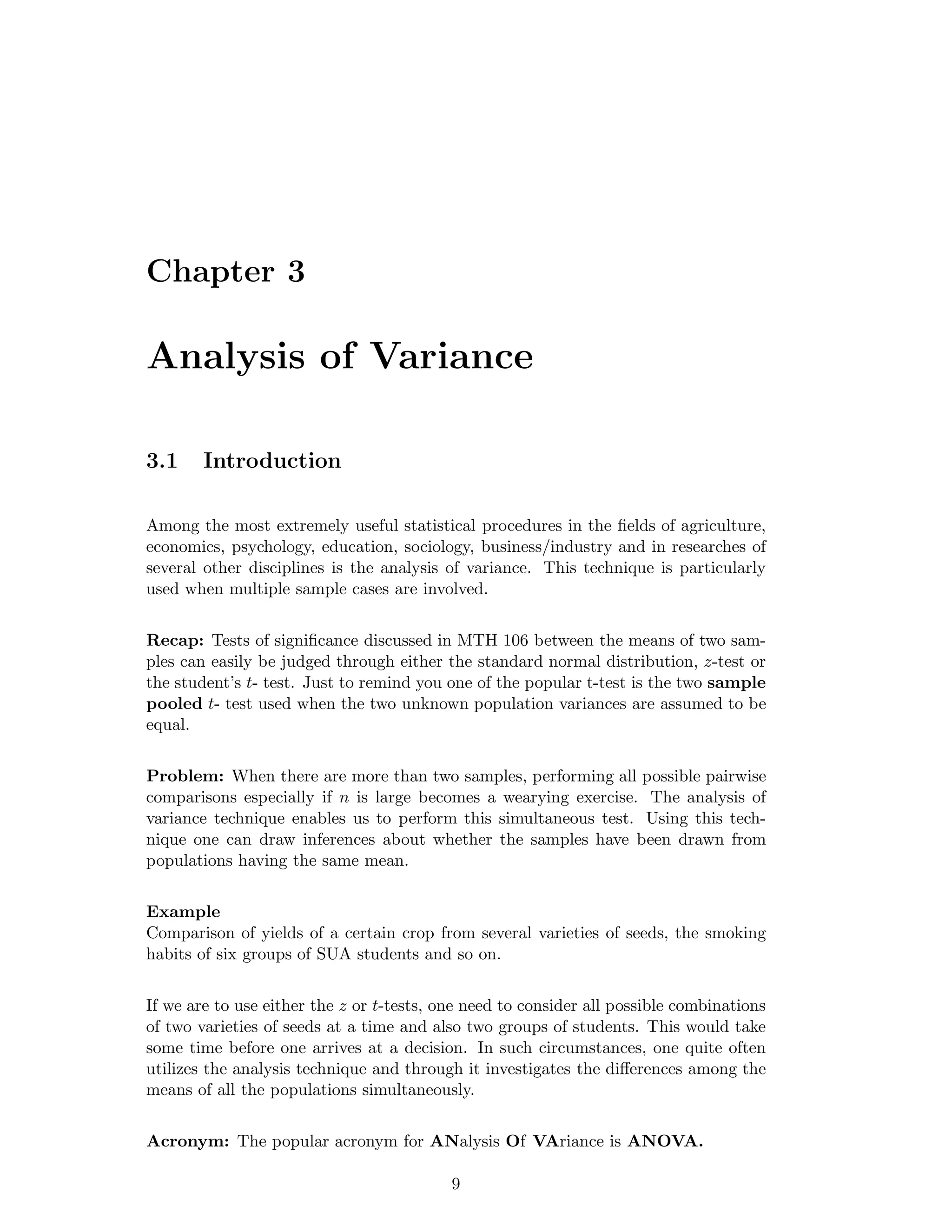
Among the most extremely useful statistical procedures in the fields of agriculture,
economics, psychology, education, sociology, business/industry and in researches of
several other disciplines is the analysis of variance. This technique is particularly
used when multiple sample cases are involved.
Recap: Tests of significance discussed in MTH 106 between the means of two sam-
ples can easily be judged through either the standard normal distribution, z-test or
the student’s t- test. Just to remind you one of the popular t-test is the two sample
pooled t- test used when the two unknown population variances are assumed to be
equal.
Problem: When there are more than two samples, performing all possible pairwise
comparisons especially if n is large becomes a wearying exercise. The analysis of
variance technique enables us to perform this simultaneous test. Using this tech-
nique one can draw inferences about whether the samples have been drawn from
populations having the same mean.
Example
Comparison of yields of a certain crop from several varieties of seeds, the smoking
habits of six groups of SUA students and so on.
If we are to use either the z or t-tests, one need to consider all possible combinations
of two varieties of seeds at a time and also two groups of students. This would take
some time before one arrives at a decision. In such circumstances, one quite often
utilizes the analysis technique and through it investigates the differences among the
means of all the populations simultaneously.
Acronym: The popular acronym for ANalysis Of VAriance is ANOVA.
9
10 CHAPTER 3. ANALYSIS OF VARIANCE
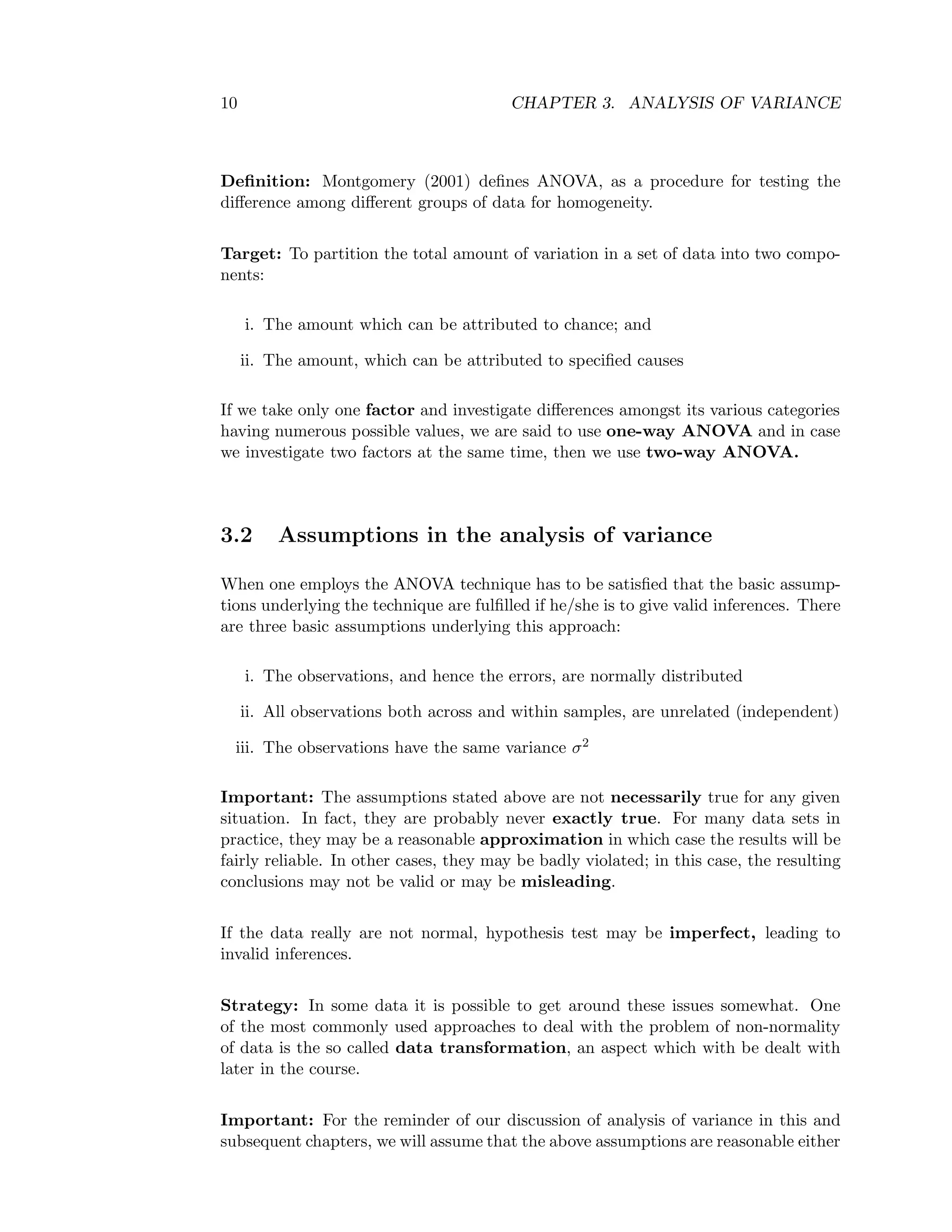
Definition: Montgomery (2001) defines ANOVA, as a procedure for testing the
difference among different groups of data for homogeneity.
Target: To partition the total amount of variation in a set of data into two compo-
nents:
i. The amount which can be attributed to chance; and
ii. The amount, which can be attributed to specified causes
If we take only one factor and investigate differences amongst its various categories
having numerous possible values, we are said to use one-way ANOVA and in case
we investigate two factors at the same time, then we use two-way ANOVA.
3.2 Assumptions in the analysis of variance
When one employs the ANOVA technique has to be satisfied that the basic assump-
tions underlying the technique are fulfilled if he/she is to give valid inferences. There
are three basic assumptions underlying this approach:
i. The observations, and hence the errors, are normally distributed
ii. All observations both across and within samples, are unrelated (independent)
iii. The observations have the same variance σ2
Important: The assumptions stated above are not necessarily true for any given
situation. In fact, they are probably never exactly true. For many data sets in
practice, they may be a reasonable approximation in which case the results will be
fairly reliable. In other cases, they may be badly violated; in this case, the resulting
conclusions may not be valid or may be misleading.
If the data really are not normal, hypothesis test may be imperfect, leading to
invalid inferences.
Strategy: In some data it is possible to get around these issues somewhat. One
of the most commonly used approaches to deal with the problem of non-normality
of data is the so called data transformation, an aspect which with be dealt with
later in the course.
Important: For the reminder of our discussion of analysis of variance in this and
subsequent chapters, we will assume that the above assumptions are reasonable either
3.3. ANALYSIS OF VARIANCE FOR ONE-WAY CLASSIFICATION 11
on the original scale of measurement of the data or transformed scale. Keep this in
mind at all times that these are just assumptions, and must be confirmed before the
methods may be considered suitable.
3.3 Analysis of variance for one-way classification
Under the one-way (or single factor) ANOVA, we randomly obtain the experimen-
tal units for the experiment and randomly assign them to the treatments so that
each experimental unit is observed under one of the treatments. In this situation,
the only way in which experimental units may be classified is with respect to which
treatment they received. Basically, the experimental units are viewed alike in this
experiment. Thus, when experimental units are thought to be alike and are thus
expected to exhibit a small amount of variation from unit to unit, grouping then
would be pointless in the sense that doing so would not add much precision to an
experiment.
It can be shown that the total variation in the observed responses can be subdivided
into two components:
i. Due to the differences in the level of factor (say A)
ii. The residual variation (error term)
3.3.1 Analysis of variance for one-way classification with unequal
replication (unbalanced data)
We will first consider the case where unequal number of replication of the treatments
to the experimental units is observed.
Notation: To facilitate the development of methods that we will require in our
discussion, we will change slightly our notation of sample mean we discussed in
MTH 106. As we will see shortly, we will be dealing with several different types of
means for the data.
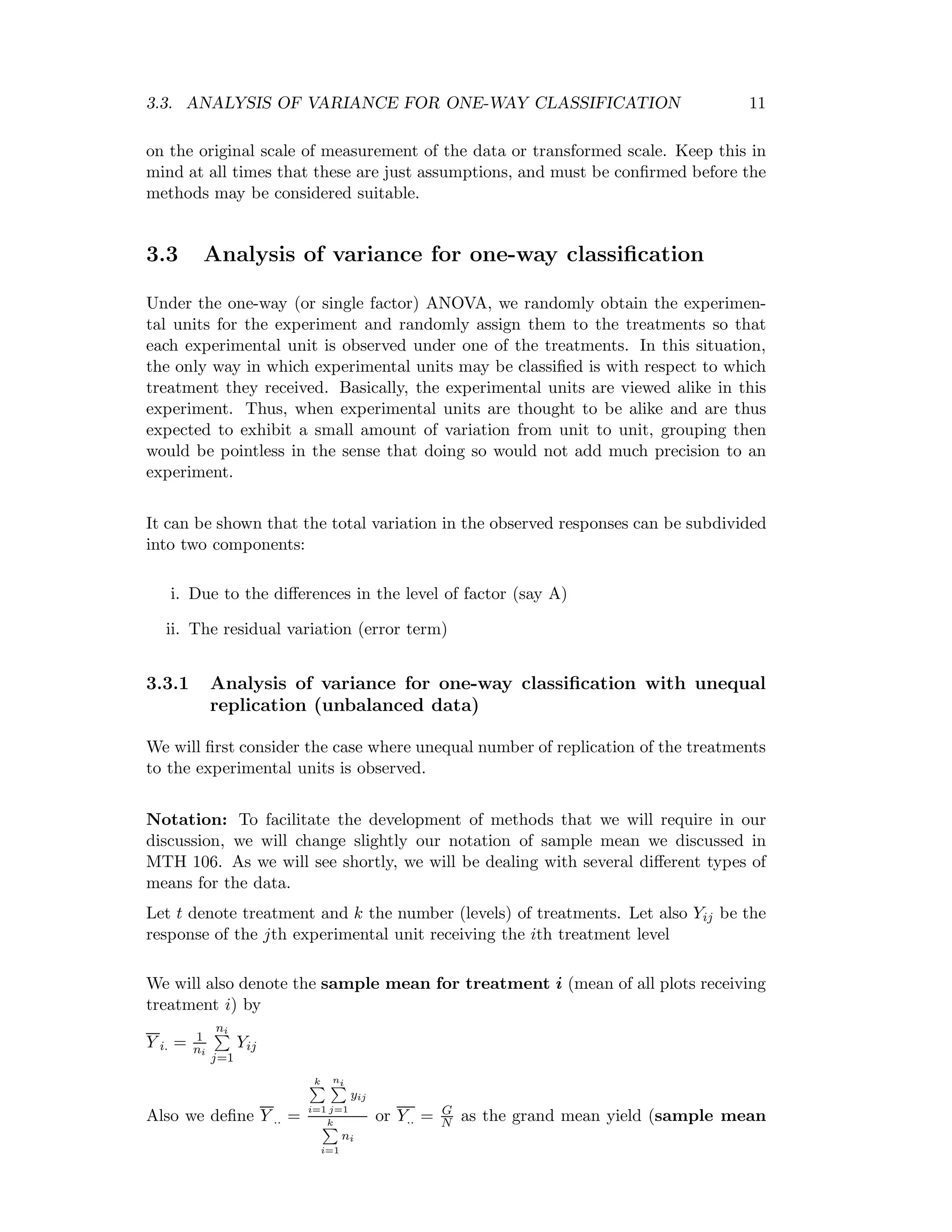
Let t denote treatment and k the number (levels) of treatments. Let also Yij be the
response of the jth experimental unit receiving the ith treatment level
We will also denote the sample mean for treatment i (mean of all plots receiving
treatment i) by
Y i. = 1
ni
ni
j=1
Yij
Also we define Y .. =
k
i=1
ni
j=1
yij
k
i=1
ni
or Y.. = G
N as the grand mean yield (sample mean
12 CHAPTER 3. ANALYSIS OF VARIANCE
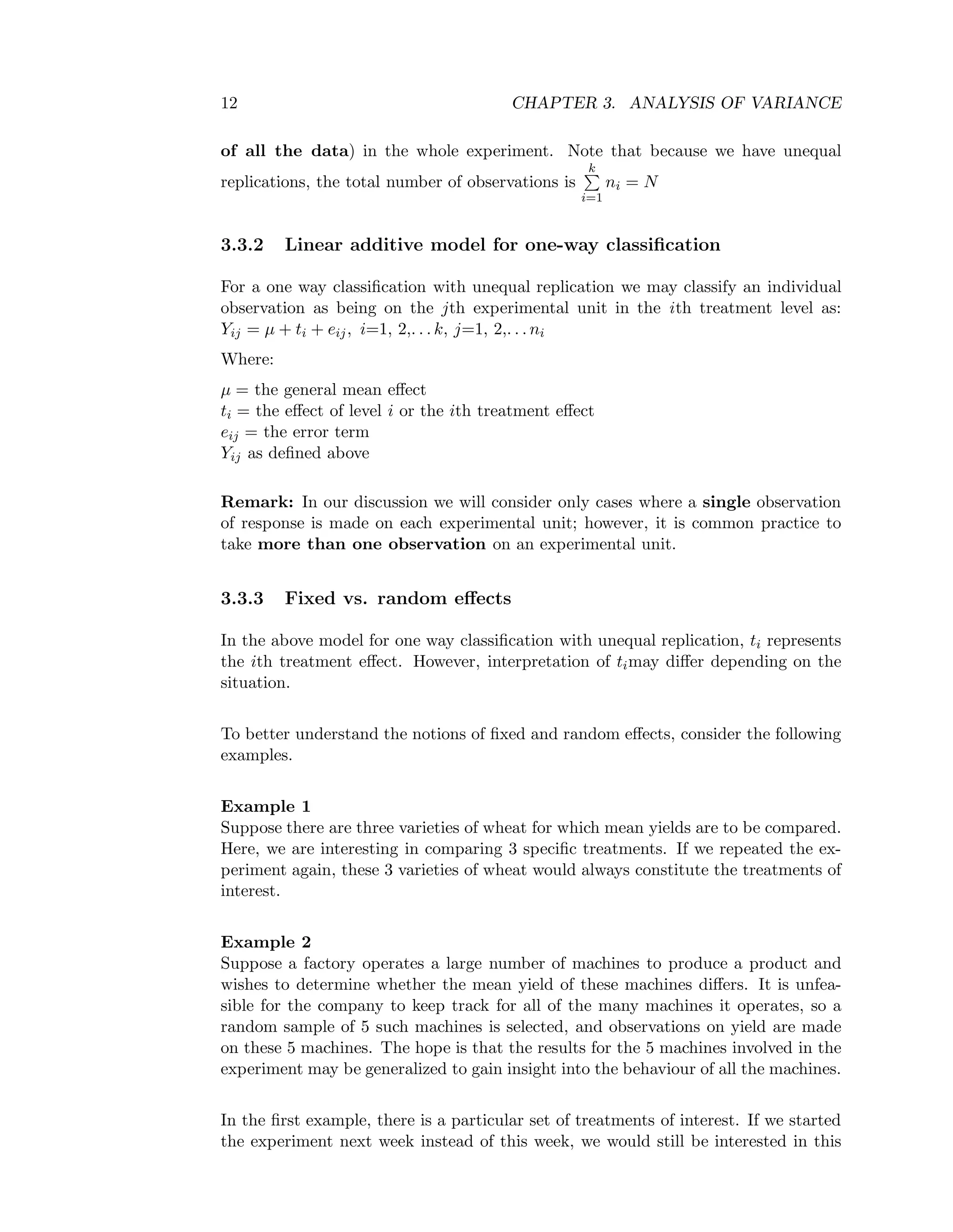
of all the data) in the whole experiment. Note that because we have unequal
replications, the total number of observations is
k
i=1
ni = N
3.3.2 Linear additive model for one-way classification
For a one way classification with unequal replication we may classify an individual
observation as being on the jth experimental unit in the ith treatment level as:
Yij = µ + ti + eij, i=1, 2,. . . k, j=1, 2,. . . ni
Where:
µ = the general mean effect
ti = the effect of level i or the ith treatment effect
eij = the error term
Yij as defined above
Remark: In our discussion we will consider only cases where a single observation
of response is made on each experimental unit; however, it is common practice to
take more than one observation on an experimental unit.
3.3.3 Fixed vs. random effects
In the above model for one way classification with unequal replication, ti represents
the ith treatment effect. However, interpretation of timay differ depending on the
situation.
To better understand the notions of fixed and random effects, consider the following
examples.
Example 1
Suppose there are three varieties of wheat for which mean yields are to be compared.
Here, we are interesting in comparing 3 specific treatments. If we repeated the ex-
periment again, these 3 varieties of wheat would always constitute the treatments of
interest.
Example 2
Suppose a factory operates a large number of machines to produce a product and
wishes to determine whether the mean yield of these machines differs. It is unfea-
sible for the company to keep track for all of the many machines it operates, so a
random sample of 5 such machines is selected, and observations on yield are made
on these 5 machines. The hope is that the results for the 5 machines involved in the
experiment may be generalized to gain insight into the behaviour of all the machines.
In the first example, there is a particular set of treatments of interest. If we started
the experiment next week instead of this week, we would still be interested in this
3.3. ANALYSIS OF VARIANCE FOR ONE-WAY CLASSIFICATION 13
same particular set of treatments. It would not vary across other possible experi-
ments we might do.
In the second example, the treatments are the 5 machines from all machines at the
company, chosen at random. If we started the experiment next week instead of this
week, we might end up with a different set of 5 machines with which to do the
experiment. Here interest focuses on the population of all machines operated by
the company. The question of interest is not about the particular treatments in the
experiment, but the population of all such treatments.
We thus make the following distinction in our model:
In the case like example 1, the ti are best regarded as fixed quantities, as they de-
scribe a particular set of conditions. Thus, ti are referred to as fixed effects
In a case like example 2, the ti are best regarded as random variables. Here the par-
ticular treatments in the experiment may be thought of as drawn from a population
of all such treatments, so there is a chance involved. In this situation, the ti are
referred to as random effects.
3.3.4 Calculation of sums of squares
As we described above, the fundamental nature of the ANOVA is that the total
amount of variation in a set of data is broken down into two components, that
amount which can be attributed to chance and that amount which can be attributed
to specified causes.
Thus, based on the above linear additive model we partition the total variation in
the data as:
Total variation = Variation due to factor A (treatment) + Residual/Error term or
Total sum of squares = Sum of squares due to factor A + Sum of squares due to error
In short we have,
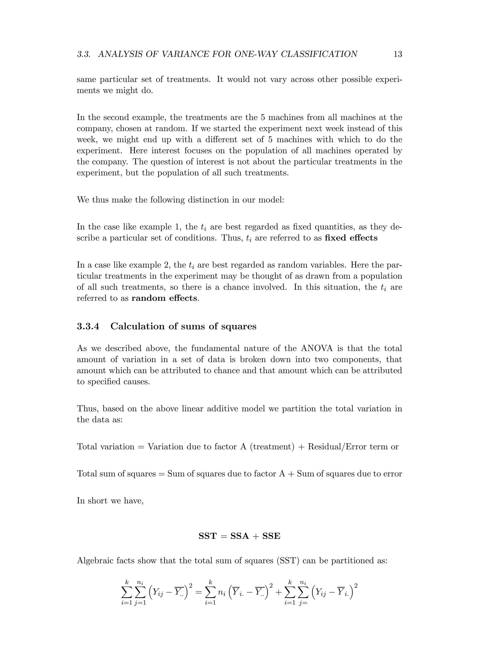
SST = SSA + SSE
Algebraic facts show that the total sum of squares (SST) can be partitioned as:
k
i=1
ni
j=1
Yij − Y..
2
=
k
i=1
ni Y i. − Y..
2
+
k
i=1
ni
j=
Yij − Y i.
2
14 CHAPTER 3. ANALYSIS OF VARIANCE
Y i.and Y .. as defined in Section 3.3.1
Thus, SST=
k
i=1
ni
j=1
Yij − Y..
2
, SSA=
k
i=1
ni
¯Yi. − ¯Y..
2
and SSE=
k
i=1
ni
j=1
Yij − ¯Yi.
2
For calculation we express the SSs as follows:
Define C.F=Correction factor =
k
i=1
ni
j=1
Yij
2
k
i=1
ni
= G2
N Here, G is the grand total=
k
i=1
ni
j=1
Yij and N as defined in Section 2.3.1
It can be shown that:
SST=
k
i=1
ni
j=
Y 2
ij −
k
i=1
ni
j=1
Yij
2
k
i=1
ni
or
k
i=1
ni
j=
Y 2
ij − G2
N or
k
i=1
ni
j=
Y 2
ij − C.F
Treatment SS or Factor A SS=
k
i=1
Y 2
i
ni
− C.F
Where: Yi =
ni
j=1
Yijis the total yield of all the njplots which carried treatment i
Error SS (SSE) =SST-SSA
Since we have k levels of factor (A) or treatment then SSA will have k-1 independent
comparisons possible (degrees of freedom). Similarly SST will have N-1 independent
comparisons (degrees of freedom), and SSE will have (N-1)-(k-1) =N−k independent
comparisons (degrees of freedom).
We summarize the computations in a table known as the ANOVA table.
Table 3.1: One way ANOVA table with unequal replication
Source of Degrees of Sum of Mean square
variation (S.V) freedom (D.F) squares (S.S) (M.S) F- ratio
Between treatments k-1 SSA SSA
K−1 = MSA MSA
MSE
Error(within treat.) N − k SSE SSE
N−k = MSE
Total N-1 SST
The calculated F-value MSA
MSE is compared with the F-tabulated value
(Fα, [(k − 1) , (N − k)]) at α level of significance for k-1 and N −k degrees of freedom.
3.3. ANALYSIS OF VARIANCE FOR ONE-WAY CLASSIFICATION 15
Statistical Hypotheses
The question of interest in this setting is to determine if the means of the different
treatment populations are different.
Mathematically we write:
Ho : µ1 = µ2 = ... = µk That is, the µi are all equal
H1 : µi = µj for at least one i = j That is, the µi are not all equal
Or simply
Ho :There is no variation among the treatments
H1 :Variation exists
Test procedure
At level of significance α, if F> Fα, [(k − 1) , (N − k)] then there is evidence for no
significance variation (i.e. we reject the null hypothesis).
Note that the alternative hypothesis stated above does not specify the way in
which the treatment means (or deviation) differ. The best we can say based on our
statistic is that they differ somehow.
Example
Four Machines are used for filling plastic bottles with a net volume of 16.0 cm3.
The quality-engineering department suspects that both machines fill to the same net
volume whether or not this volume is 16.0 cm3. A random sample is taken from the
output of each machine.
Table 3.2: Machine data set
Machines
A B C D
16.03 16.01 16.02 16.03
16.04 15.99 15.97 16.04
15.96 16.03 15.96 16.00
16.05 15.05 16.02
16.04
Total 64.08 48.03 79.04 64.09
Assume that the measurements are approximately normally distributed, with ap-
proximately constant variance σ2. Do you think the quality-engineering department
is correct? Use α = 0.05
Statistical hypotheses:
Ho :There is no significant variation among the levels of machines
H1 :Variation exists
or
Ho : µ1 = µ2 = µ3 = µ4 (all means are equal)
16 CHAPTER 3. ANALYSIS OF VARIANCE
H1 : µi = µj for at least one i = j (the means are not all equal)
Calculation
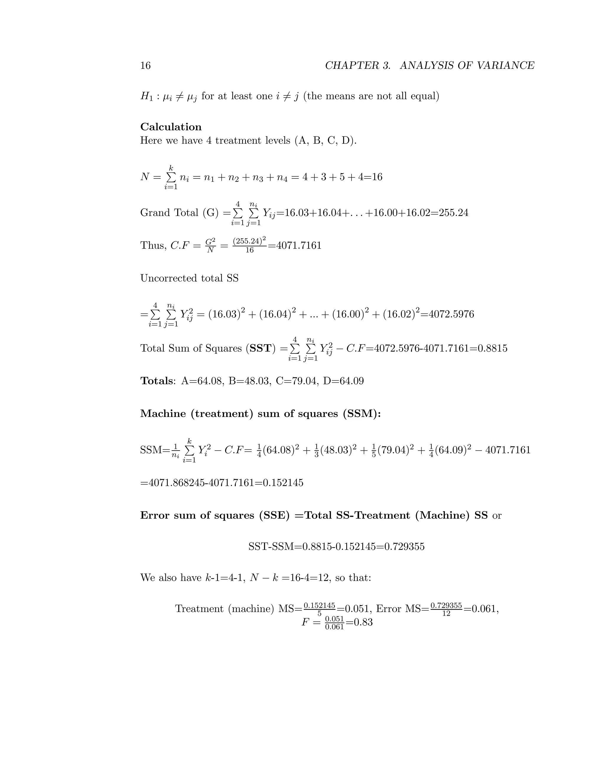
Here we have 4 treatment levels (A, B, C, D).
N =
k
i=1
ni = n1 + n2 + n3 + n4 = 4 + 3 + 5 + 4=16
Grand Total (G) =
4
i=1
ni
j=1
Yij=16.03+16.04+. . . +16.00+16.02=255.24
Thus, C.F = G2
N = (255.24)2
16 =4071.7161
Uncorrected total SS
=
4
i=1
ni
j=1
Y 2
ij = (16.03)2
+ (16.04)2
+ ... + (16.00)2
+ (16.02)2
=4072.5976
Total Sum of Squares (SST) =
4
i=1
ni
j=1
Y 2
ij − C.F=4072.5976-4071.7161=0.8815
Totals: A=64.08, B=48.03, C=79.04, D=64.09
Machine (treatment) sum of squares (SSM):
SSM= 1
ni
k
i=1
Y 2
i − C.F= 1
4(64.08)2 + 1
3(48.03)2 + 1
5(79.04)2 + 1
4(64.09)2 − 4071.7161
=4071.868245-4071.7161=0.152145
Error sum of squares (SSE) =Total SS-Treatment (Machine) SS or
SST-SSM=0.8815-0.152145=0.729355
We also have k-1=4-1, N − k =16-4=12, so that:
Treatment (machine) MS=0.152145
5 =0.051, Error MS=0.729355
12 =0.061,
F = 0.051
0.061 =0.83
3.3. ANALYSIS OF VARIANCE FOR ONE-WAY CLASSIFICATION 17
We summarize the computation in an analysis of variance table:
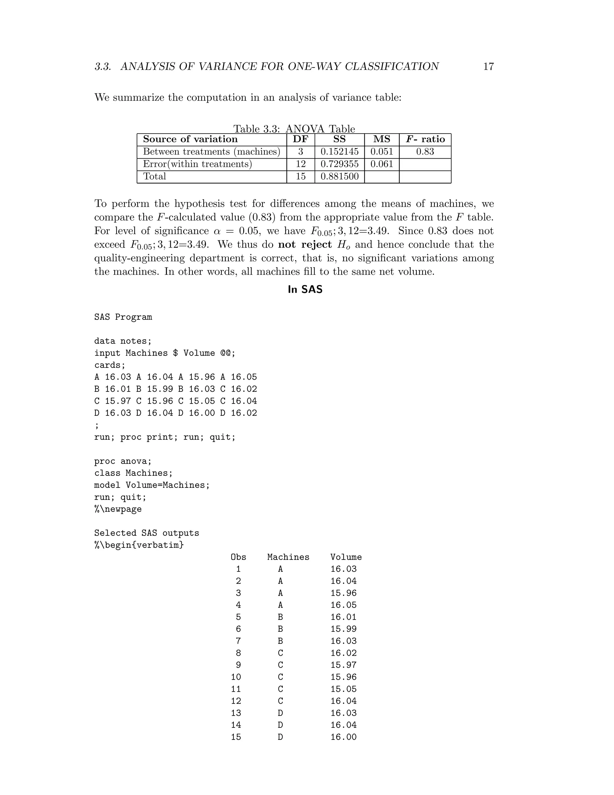
Table 3.3: ANOVA Table
Source of variation DF SS MS F- ratio
Between treatments (machines) 3 0.152145 0.051 0.83
Error(within treatments) 12 0.729355 0.061
Total 15 0.881500
To perform the hypothesis test for differences among the means of machines, we
compare the F-calculated value (0.83) from the appropriate value from the F table.
For level of significance α = 0.05, we have F0.05; 3, 12=3.49. Since 0.83 does not
exceed F0.05; 3, 12=3.49. We thus do not reject Ho and hence conclude that the
quality-engineering department is correct, that is, no significant variations among
the machines. In other words, all machines fill to the same net volume.
In SAS
SAS Program
data notes;
input Machines $ Volume @@;
cards;
A 16.03 A 16.04 A 15.96 A 16.05
B 16.01 B 15.99 B 16.03 C 16.02
C 15.97 C 15.96 C 15.05 C 16.04
D 16.03 D 16.04 D 16.00 D 16.02
;
run; proc print; run; quit;
proc anova;
class Machines;
model Volume=Machines;
run; quit;
%newpage
Selected SAS outputs
%begin{verbatim}
Obs Machines Volume
1 A 16.03
2 A 16.04
3 A 15.96
4 A 16.05
5 B 16.01
6 B 15.99
7 B 16.03
8 C 16.02
9 C 15.97
10 C 15.96
11 C 15.05
12 C 16.04
13 D 16.03
14 D 16.04
15 D 16.00
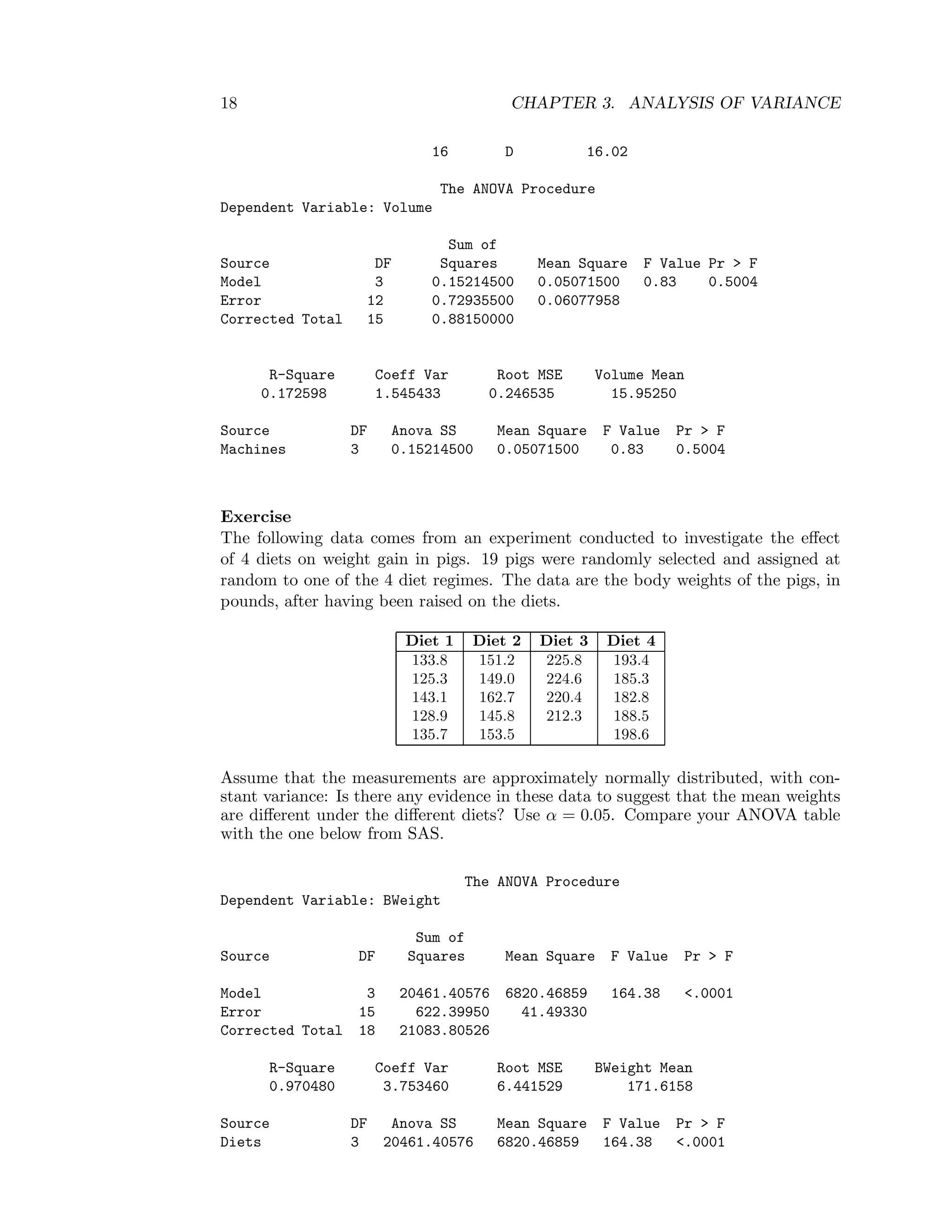
18 CHAPTER 3. ANALYSIS OF VARIANCE
16 D 16.02
The ANOVA Procedure
Dependent Variable: Volume
Sum of
Source DF Squares Mean Square F Value Pr > F
Model 3 0.15214500 0.05071500 0.83 0.5004
Error 12 0.72935500 0.06077958
Corrected Total 15 0.88150000
R-Square Coeff Var Root MSE Volume Mean
0.172598 1.545433 0.246535 15.95250
Source DF Anova SS Mean Square F Value Pr > F
Machines 3 0.15214500 0.05071500 0.83 0.5004
Exercise
The following data comes from an experiment conducted to investigate the effect
of 4 diets on weight gain in pigs. 19 pigs were randomly selected and assigned at
random to one of the 4 diet regimes. The data are the body weights of the pigs, in
pounds, after having been raised on the diets.
Diet 1 Diet 2 Diet 3 Diet 4
133.8 151.2 225.8 193.4
125.3 149.0 224.6 185.3
143.1 162.7 220.4 182.8
128.9 145.8 212.3 188.5
135.7 153.5 198.6
Assume that the measurements are approximately normally distributed, with con-
stant variance: Is there any evidence in these data to suggest that the mean weights
are different under the different diets? Use α = 0.05. Compare your ANOVA table
with the one below from SAS.
The ANOVA Procedure
Dependent Variable: BWeight
Sum of
Source DF Squares Mean Square F Value Pr > F
Model 3 20461.40576 6820.46859 164.38 <.0001
Error 15 622.39950 41.49330
Corrected Total 18 21083.80526
R-Square Coeff Var Root MSE BWeight Mean
0.970480 3.753460 6.441529 171.6158
Source DF Anova SS Mean Square F Value Pr > F
Diets 3 20461.40576 6820.46859 164.38 <.0001
3.3. ANALYSIS OF VARIANCE FOR ONE-WAY CLASSIFICATION 19
3.3.5 ANOVA for one-way classification with equal replication (bal-
anced data)
In the above exercise the diets 1, 2, and 4 are each replicated 5 times while diet 3 is
replicated 4 times. In this case as we have discussed above, the sample mean for
treatment i is Y i. = 1
ni
ni
j=1
Yij. We now discuss the case where ni = n for all i,
i=1, 2,. . . , k
Since each treatment is replicated the same number of time (say n), then the total
number of observations, N=nk.
Thus, with this new notation, we define the quantities Y i.,Y .., Total SS, Treatment
SS, and Error SS and their degrees of freedom as follows:
Y i. = 1
n
n
j=1
Yij, Y .. =
k
i=1
n
j=1
yij
nk orY.. = G
N , Total SS (SST) =
k
i=1
n
j=1
Y 2
ij − G2
N ,
Treatment SS or Factor A SS=
k
i=1
Y 2
i
n − C.F where C.F =
k
i=1
n
j=1
Yij
2
nk = G2
N
G = the grand total=
k
i=1
n
j=1
Yij
The degrees of freedom for Treatment SS, Error SS and Total SS, are respectively
(k-1), (N − k) or (nk-k) or k(n-1) and (N-1) or (nk-1).
Table 3.4: One way ANOVA table with equal replication
Source of DF SS MS F- ratio
variation
Between treat. k-1 SSA SSA
k−1 = MSA MSA
MSE
Error (within treat.) k(n-1) SSE SSE
k(n−1) = MSE
Total N-1 SST
The calculated F-value MSA
MSE is compared with the F-tabulated value
(Fα, [(k − 1) , (k(n − 1))]) at α level of significance for k-1 and k(n-1) degrees of free-
dom.
Statistical Hypotheses as given above
Test procedure
At level of significanceα, if F> Fα, [(k − 1) , (k(n − 1))] then there is evidence for no
significance variation (i.e. we reject the null hypothesis).
Example
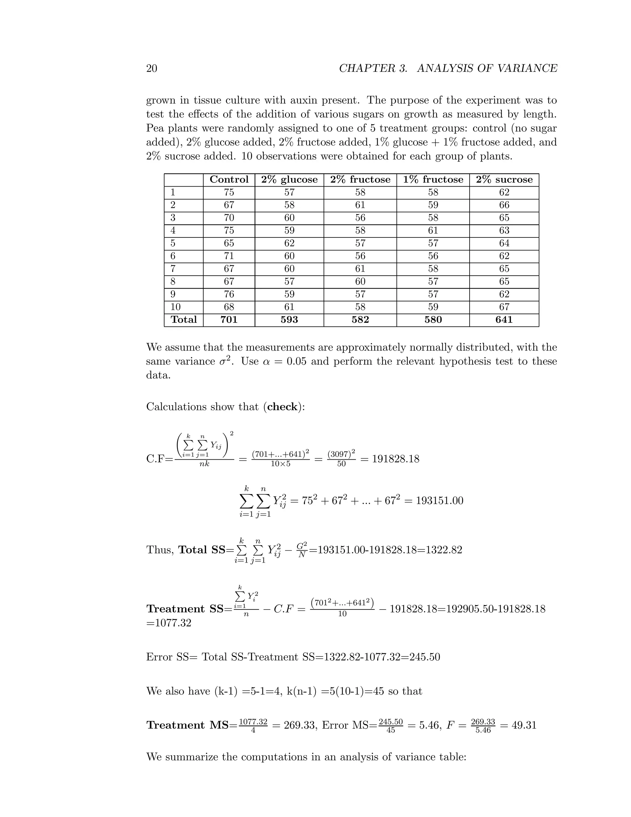
The following data record the length of pea sections, in ocular units (×0.114 mm),
20 CHAPTER 3. ANALYSIS OF VARIANCE
grown in tissue culture with auxin present. The purpose of the experiment was to
test the effects of the addition of various sugars on growth as measured by length.
Pea plants were randomly assigned to one of 5 treatment groups: control (no sugar
added), 2% glucose added, 2% fructose added, 1% glucose + 1% fructose added, and
2% sucrose added. 10 observations were obtained for each group of plants.
Control 2% glucose 2% fructose 1% fructose 2% sucrose
1 75 57 58 58 62
2 67 58 61 59 66
3 70 60 56 58 65
4 75 59 58 61 63
5 65 62 57 57 64
6 71 60 56 56 62
7 67 60 61 58 65
8 67 57 60 57 65
9 76 59 57 57 62
10 68 61 58 59 67
Total 701 593 582 580 641
We assume that the measurements are approximately normally distributed, with the
same variance σ2. Use α = 0.05 and perform the relevant hypothesis test to these
data.
Calculations show that (check):
C.F=
k
i=1
n
j=1
Yij
2
nk = (701+...+641)2
10×5 = (3097)2
50 = 191828.18
k
i=1
n
j=1
Y 2
ij = 752
+ 672
+ ... + 672
= 193151.00
Thus, Total SS=
k
i=1
n
j=1
Y 2
ij − G2
N =193151.00-191828.18=1322.82
Treatment SS=
k
i=1
Y 2
i
n − C.F =
(7012+...+6412
)
10 − 191828.18=192905.50-191828.18
=1077.32
Error SS= Total SS-Treatment SS=1322.82-1077.32=245.50
We also have (k-1) =5-1=4, k(n-1) =5(10-1)=45 so that
Treatment MS=1077.32
4 = 269.33, Error MS=245.50
45 = 5.46, F = 269.33
5.46 = 49.31
We summarize the computations in an analysis of variance table:
3.4. ANOVA FOR TWO-WAY CLASSIFICATION (WITHOUT REPLICATION)21
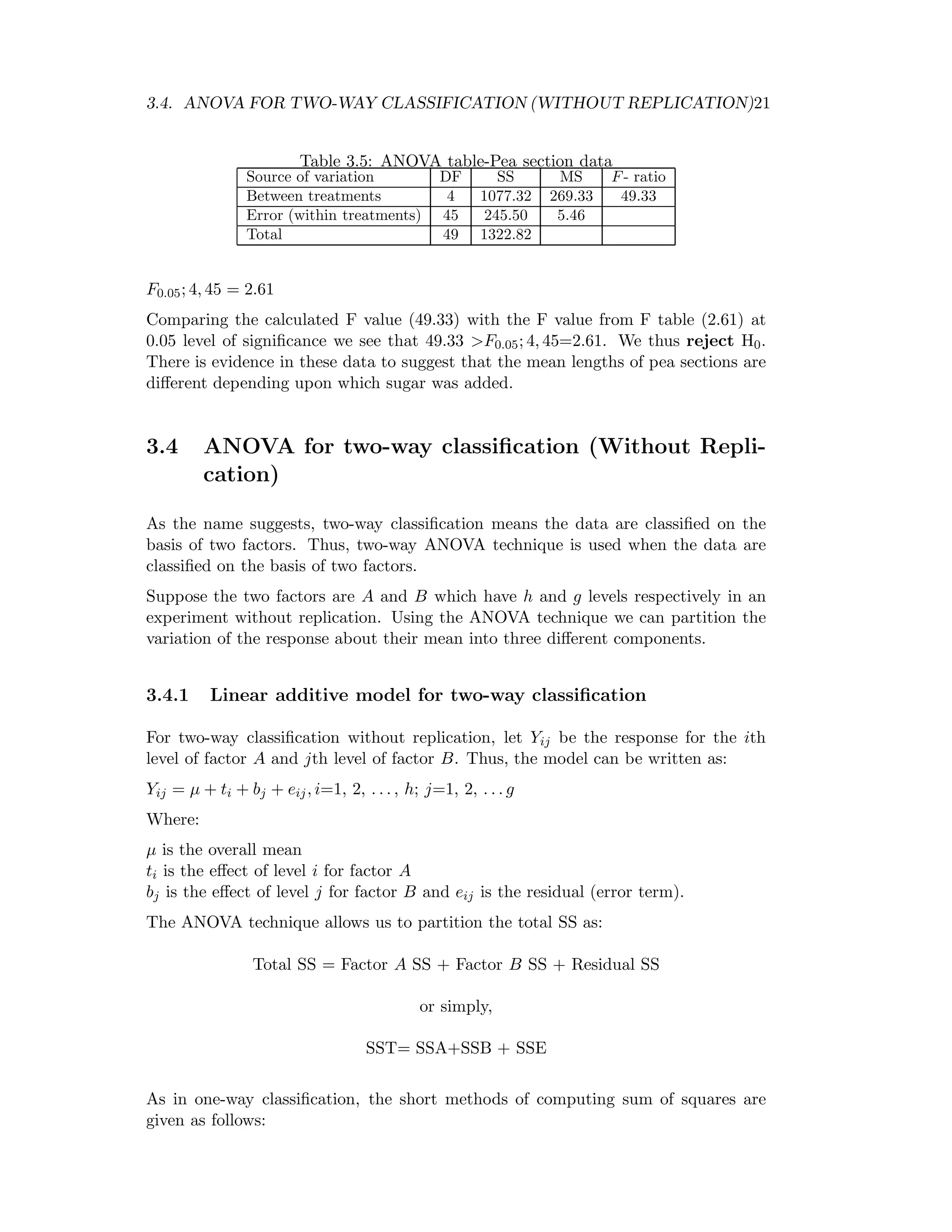
Table 3.5: ANOVA table-Pea section data
Source of variation DF SS MS F- ratio
Between treatments 4 1077.32 269.33 49.33
Error (within treatments) 45 245.50 5.46
Total 49 1322.82
F0.05; 4, 45 = 2.61
Comparing the calculated F value (49.33) with the F value from F table (2.61) at
0.05 level of significance we see that 49.33 >F0.05; 4, 45=2.61. We thus reject H0.
There is evidence in these data to suggest that the mean lengths of pea sections are
different depending upon which sugar was added.
3.4 ANOVA for two-way classification (Without Repli-
cation)
As the name suggests, two-way classification means the data are classified on the
basis of two factors. Thus, two-way ANOVA technique is used when the data are
classified on the basis of two factors.
Suppose the two factors are A and B which have h and g levels respectively in an
experiment without replication. Using the ANOVA technique we can partition the
variation of the response about their mean into three different components.
3.4.1 Linear additive model for two-way classification
For two-way classification without replication, let Yij be the response for the ith
level of factor A and jth level of factor B. Thus, the model can be written as:
Yij = µ + ti + bj + eij, i=1, 2, . . . , h; j=1, 2, . . . g
Where:
µ is the overall mean
ti is the effect of level i for factor A
bj is the effect of level j for factor B and eij is the residual (error term).
The ANOVA technique allows us to partition the total SS as:
Total SS = Factor A SS + Factor B SS + Residual SS
or simply,
SST= SSA+SSB + SSE
As in one-way classification, the short methods of computing sum of squares are
given as follows:
22 CHAPTER 3. ANALYSIS OF VARIANCE
Let N (=hg) be the total number of experimental observations
Let G = the sum of yields over all the N (=hg) plots. So that G =
h
i=1
g
j=
Yij,
Correction factor (C.F) =G2
N =
h
i=1
g
j=1
Yij
2
hg
Total SS (SST) =
h
i=1
g
j=1
Y 2
ij − C.F
Factor A SS (SSA) =1
g
h
i=1
Y 2
i − C.F where Yi =
g
j=1
Yij is the total yield of all the
g plots which carried treatment i.
Factor B SS (SSB) =1
h
g
j=1
Y 2
j − C.F where Yj =
h
i=1
Yij is the total yield of all
the h plots which carried treatment j.
Error SS (SSE) = SST – (SSA +SSB)= SST –SSA- SSB
Table 3.6: ANOVA table for two-way classification
Source of variation DF SS MS F-ratio
Factor A h-1 SSA SSA
h−1 = MSA MSA
MSE
Factor B g-1 SSB SSB
g−1 = MSB MSB
MSE
Residual (h-1)(g-1) SSE SSE
(h−1)(g−1) = MSE
Total N-1 SST
Statistical hypotheses:
Factor A:
Ho: t1 = t2=. . . =th
H1: ti =tj for at least one i = j
Factor B:
Ho: b1=b2=. . . =bg
H1: bi =bj for at least one i = j
Test procedure
Reject Ho for factor A, if the calculated F-value MSA
MSE > the tabulated F-value
Fα, [(h − 1) , (h − 1)(g − 1)] at α-level of significance. Otherwise, we do not reject
Ho.
Similarly, reject Ho for factor B, if the calculated F-value MSB
MSE > the tabulated
F-value Fα, [(g − 1) , (h − 1)(g − 1)] at α-level of significance. Otherwise, we do not
reject Ho
3.4. ANOVA FOR TWO-WAY CLASSIFICATION (WITHOUT REPLICATION)23
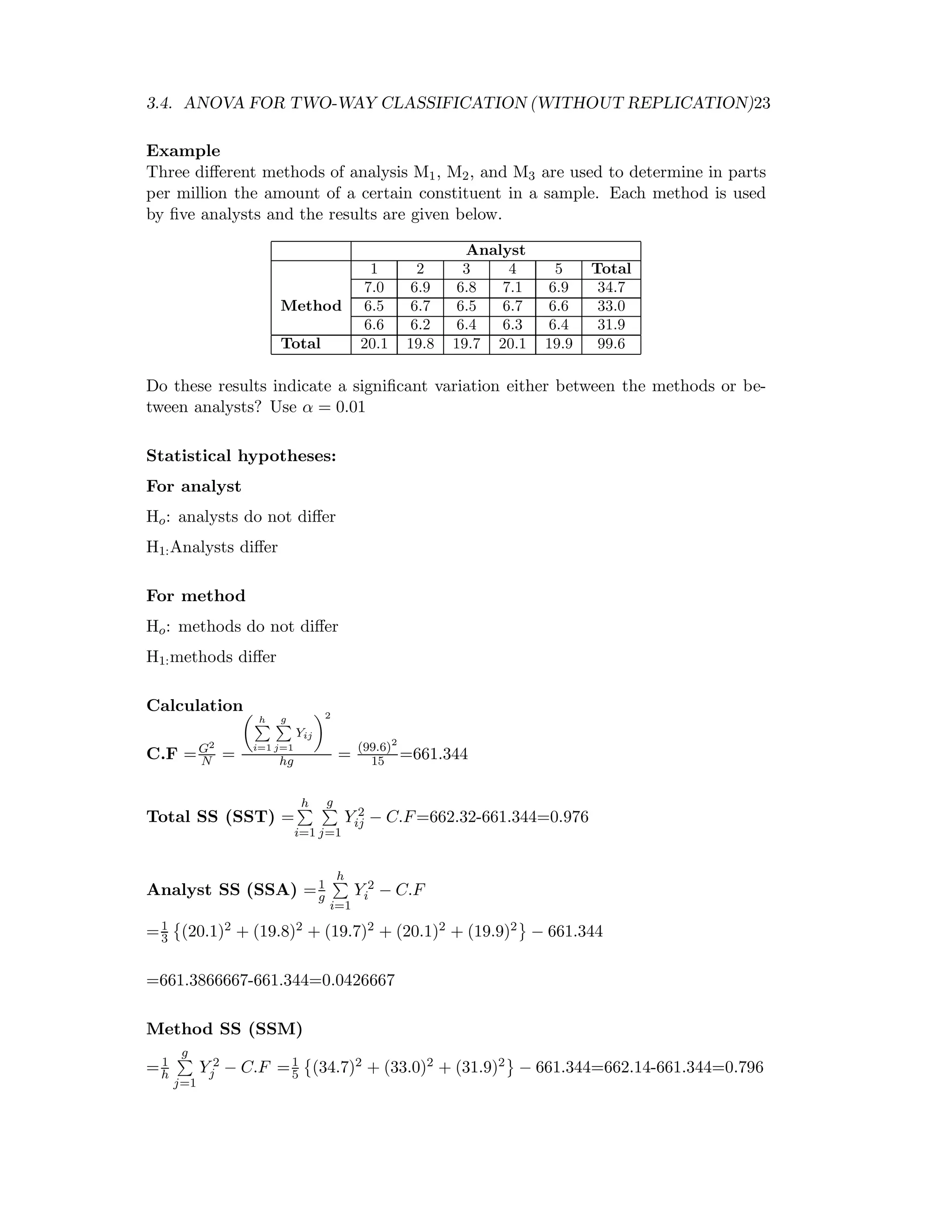
Example
Three different methods of analysis M1, M2, and M3 are used to determine in parts
per million the amount of a certain constituent in a sample. Each method is used
by five analysts and the results are given below.
Analyst
1 2 3 4 5 Total
7.0 6.9 6.8 7.1 6.9 34.7
Method 6.5 6.7 6.5 6.7 6.6 33.0
6.6 6.2 6.4 6.3 6.4 31.9
Total 20.1 19.8 19.7 20.1 19.9 99.6
Do these results indicate a significant variation either between the methods or be-
tween analysts? Use α = 0.01
Statistical hypotheses:
For analyst
Ho: analysts do not differ
H1:Analysts differ
For method
Ho: methods do not differ
H1:methods differ
Calculation
C.F =G2
N =
h
i=1
g
j=1
Yij
2
hg = (99.6)2
15 =661.344
Total SS (SST) =
h
i=1
g
j=1
Y 2
ij − C.F=662.32-661.344=0.976
Analyst SS (SSA) =1
g
h
i=1
Y 2
i − C.F
=1
3 (20.1)2 + (19.8)2 + (19.7)2 + (20.1)2 + (19.9)2 − 661.344
=661.3866667-661.344=0.0426667
Method SS (SSM)
=1
h
g
j=1
Y 2
j − C.F =1
5 (34.7)2 + (33.0)2 + (31.9)2 − 661.344=662.14-661.344=0.796
24 CHAPTER 3. ANALYSIS OF VARIANCE
Error SS (SSE):
= SST –SSA- SSM=0.976-0.0426667-0.796=0.1373333
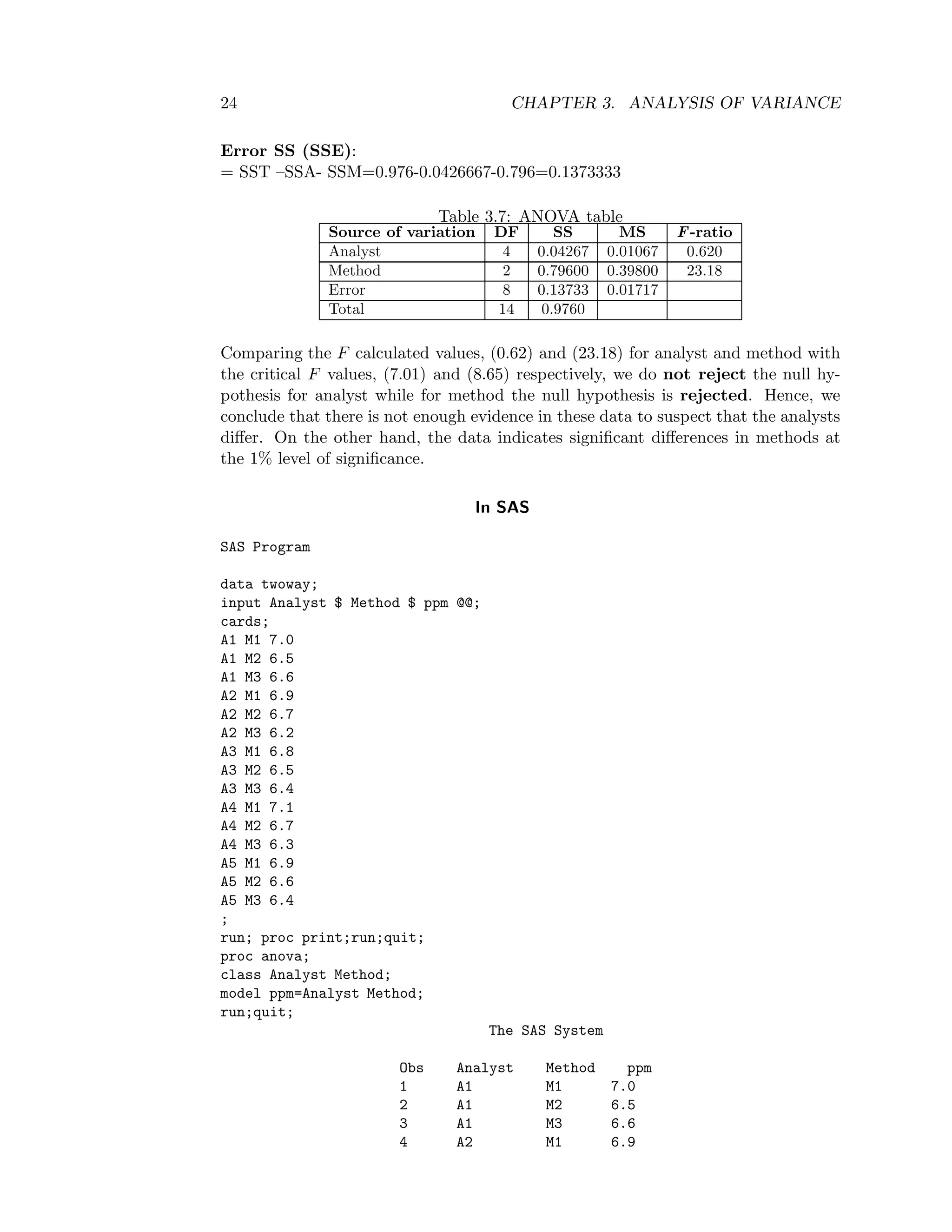
Table 3.7: ANOVA table
Source of variation DF SS MS F-ratio
Analyst 4 0.04267 0.01067 0.620
Method 2 0.79600 0.39800 23.18
Error 8 0.13733 0.01717
Total 14 0.9760
Comparing the F calculated values, (0.62) and (23.18) for analyst and method with
the critical F values, (7.01) and (8.65) respectively, we do not reject the null hy-
pothesis for analyst while for method the null hypothesis is rejected. Hence, we
conclude that there is not enough evidence in these data to suspect that the analysts
differ. On the other hand, the data indicates significant differences in methods at
the 1% level of significance.
In SAS
SAS Program
data twoway;
input Analyst $ Method $ ppm @@;
cards;
A1 M1 7.0
A1 M2 6.5
A1 M3 6.6
A2 M1 6.9
A2 M2 6.7
A2 M3 6.2
A3 M1 6.8
A3 M2 6.5
A3 M3 6.4
A4 M1 7.1
A4 M2 6.7
A4 M3 6.3
A5 M1 6.9
A5 M2 6.6
A5 M3 6.4
;
run; proc print;run;quit;
proc anova;
class Analyst Method;
model ppm=Analyst Method;
run;quit;
The SAS System
Obs Analyst Method ppm
1 A1 M1 7.0
2 A1 M2 6.5
3 A1 M3 6.6
4 A2 M1 6.9
3.5. THE LEAST SIGNIFICANCE DIFFERENCE (LSD) 25
5 A2 M2 6.7
6 A2 M3 6.2
7 A3 M1 6.8
. . . .
. . . .
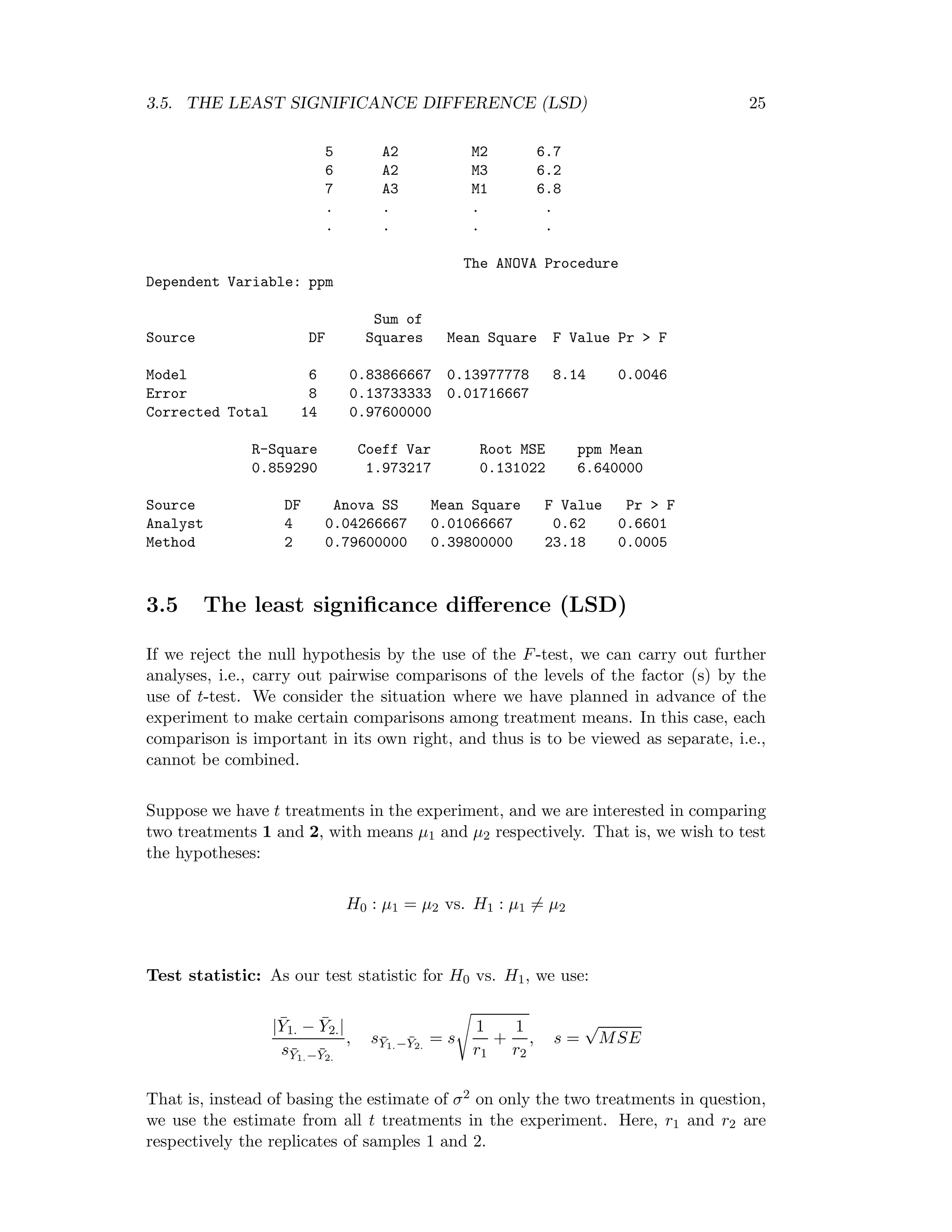
The ANOVA Procedure
Dependent Variable: ppm
Sum of
Source DF Squares Mean Square F Value Pr > F
Model 6 0.83866667 0.13977778 8.14 0.0046
Error 8 0.13733333 0.01716667
Corrected Total 14 0.97600000
R-Square Coeff Var Root MSE ppm Mean
0.859290 1.973217 0.131022 6.640000
Source DF Anova SS Mean Square F Value Pr > F
Analyst 4 0.04266667 0.01066667 0.62 0.6601
Method 2 0.79600000 0.39800000 23.18 0.0005
3.5 The least significance difference (LSD)
If we reject the null hypothesis by the use of the F-test, we can carry out further
analyses, i.e., carry out pairwise comparisons of the levels of the factor (s) by the
use of t-test. We consider the situation where we have planned in advance of the
experiment to make certain comparisons among treatment means. In this case, each
comparison is important in its own right, and thus is to be viewed as separate, i.e.,
cannot be combined.
Suppose we have t treatments in the experiment, and we are interested in comparing
two treatments 1 and 2, with means µ1 and µ2 respectively. That is, we wish to test
the hypotheses:
H0 : µ1 = µ2 vs. H1 : µ1 = µ2
Test statistic: As our test statistic for H0 vs. H1, we use:
| ¯Y1. − ¯Y2.|
s¯Y1.− ¯Y2.
, s¯Y1.− ¯Y2.
= s
1
r1
+
1
r2
, s =
√
MSE
That is, instead of basing the estimate of σ2 on only the two treatments in question,
we use the estimate from all t treatments in the experiment. Here, r1 and r2 are
respectively the replicates of samples 1 and 2.
26 CHAPTER 3. ANALYSIS OF VARIANCE
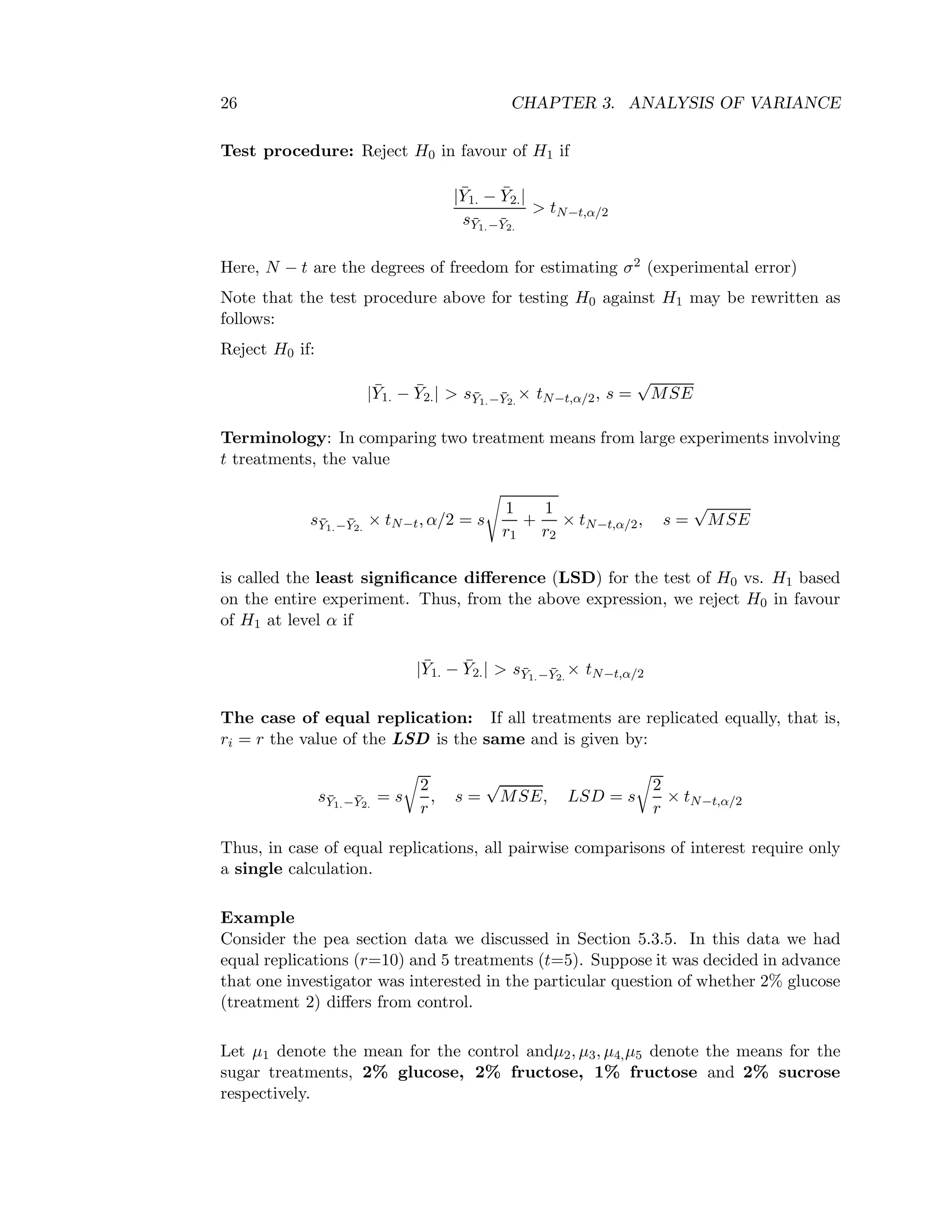
Test procedure: Reject H0 in favour of H1 if
| ¯Y1. − ¯Y2.|
s¯Y1.− ¯Y2.
> tN−t,α/2
Here, N − t are the degrees of freedom for estimating σ2 (experimental error)
Note that the test procedure above for testing H0 against H1 may be rewritten as
follows:
Reject H0 if:
| ¯Y1. − ¯Y2.| > s¯Y1.− ¯Y2.
× tN−t,α/2, s =
√
MSE
Terminology: In comparing two treatment means from large experiments involving
t treatments, the value
s¯Y1.− ¯Y2.
× tN−t, α/2 = s
1
r1
+
1
r2
× tN−t,α/2, s =
√
MSE
is called the least significance difference (LSD) for the test of H0 vs. H1 based
on the entire experiment. Thus, from the above expression, we reject H0 in favour
of H1 at level α if
| ¯Y1. − ¯Y2.| > s¯Y1.− ¯Y2.
× tN−t,α/2
The case of equal replication: If all treatments are replicated equally, that is,
ri = r the value of the LSD is the same and is given by:
s¯Y1.− ¯Y2.
= s
2
r
, s =
√
MSE, LSD = s
2
r
× tN−t,α/2
Thus, in case of equal replications, all pairwise comparisons of interest require only
a single calculation.
Example
Consider the pea section data we discussed in Section 5.3.5. In this data we had
equal replications (r=10) and 5 treatments (t=5). Suppose it was decided in advance
that one investigator was interested in the particular question of whether 2% glucose
(treatment 2) differs from control.
Let µ1 denote the mean for the control andµ2, µ3, µ4,µ5 denote the means for the
sugar treatments, 2% glucose, 2% fructose, 1% fructose and 2% sucrose
respectively.
3.5. THE LEAST SIGNIFICANCE DIFFERENCE (LSD) 27
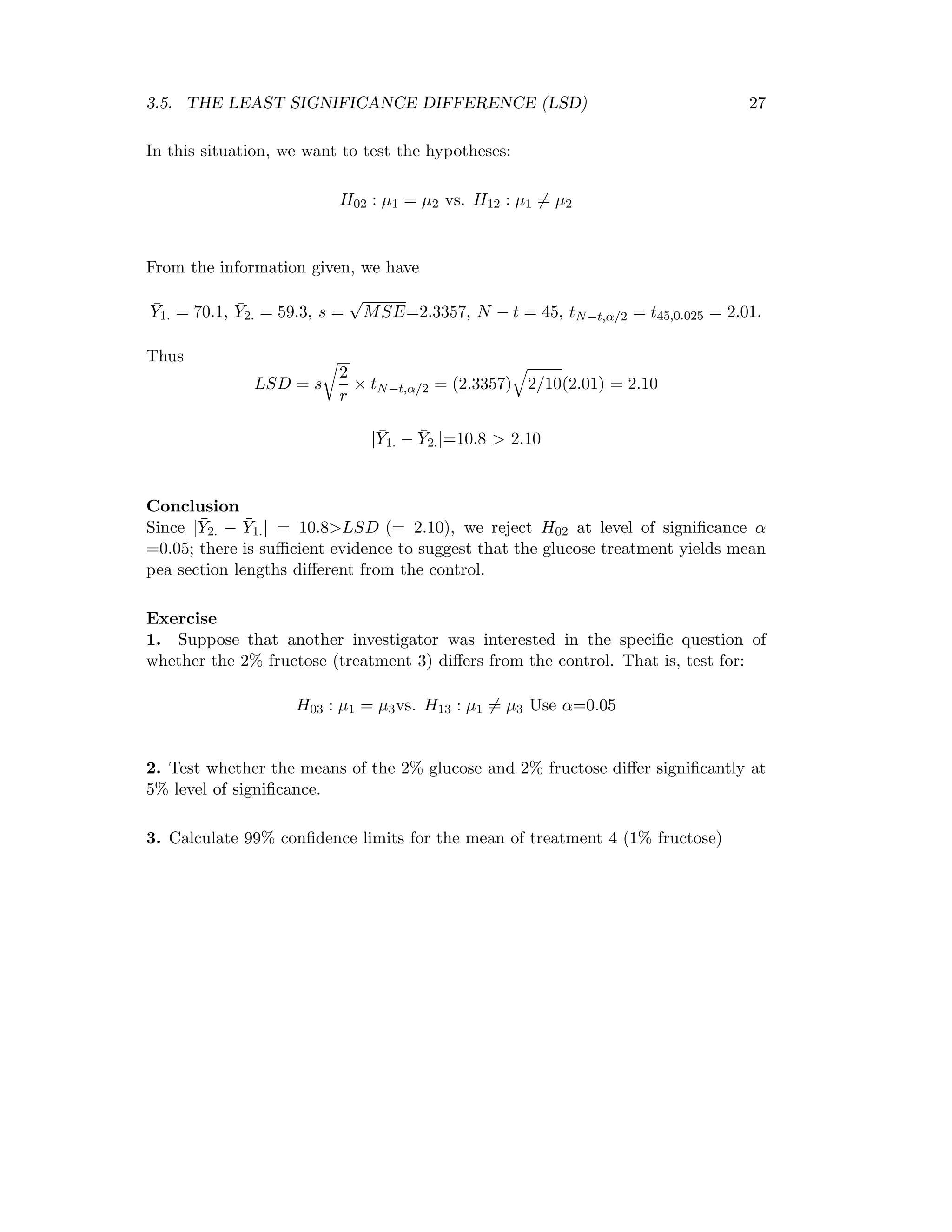
In this situation, we want to test the hypotheses:
H02 : µ1 = µ2 vs. H12 : µ1 = µ2
From the information given, we have
¯Y1. = 70.1, ¯Y2. = 59.3, s =
√
MSE=2.3357, N − t = 45, tN−t,α/2 = t45,0.025 = 2.01.
Thus
LSD = s
2
r
× tN−t,α/2 = (2.3357) 2/10(2.01) = 2.10
| ¯Y1. − ¯Y2.|=10.8 > 2.10
Conclusion
Since | ¯Y2. − ¯Y1.| = 10.8>LSD (= 2.10), we reject H02 at level of significance α
=0.05; there is sufficient evidence to suggest that the glucose treatment yields mean
pea section lengths different from the control.
Exercise
1. Suppose that another investigator was interested in the specific question of
whether the 2% fructose (treatment 3) differs from the control. That is, test for:
H03 : µ1 = µ3vs. H13 : µ1 = µ3 Use α=0.05
2. Test whether the means of the 2% glucose and 2% fructose differ significantly at
5% level of significance.
3. Calculate 99% confidence limits for the mean of treatment 4 (1% fructose)
28 CHAPTER 3. ANALYSIS OF VARIANCE
Chapter 4
Introduction to SPSS
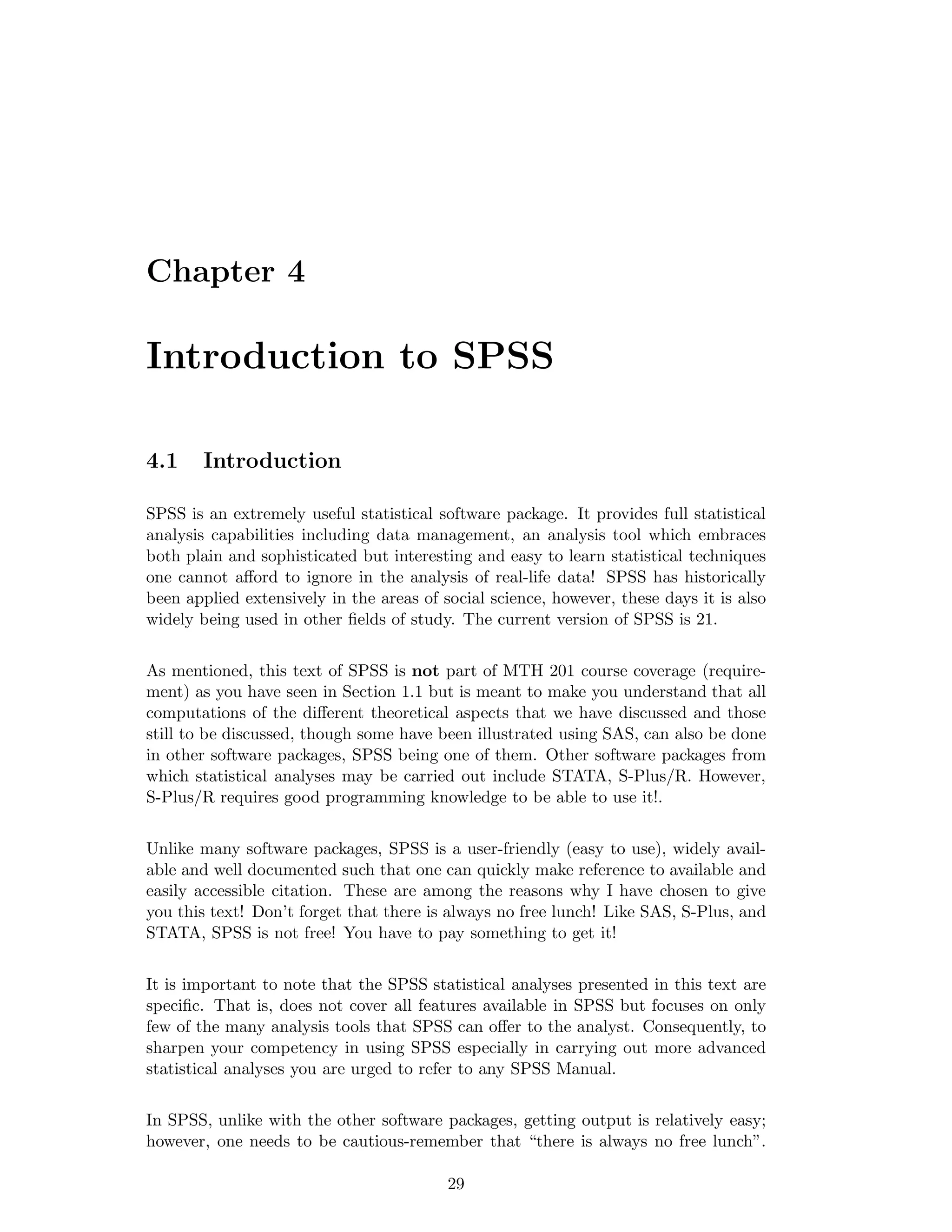
4.1 Introduction
SPSS is an extremely useful statistical software package. It provides full statistical
analysis capabilities including data management, an analysis tool which embraces
both plain and sophisticated but interesting and easy to learn statistical techniques
one cannot afford to ignore in the analysis of real-life data! SPSS has historically
been applied extensively in the areas of social science, however, these days it is also
widely being used in other fields of study. The current version of SPSS is 21.
As mentioned, this text of SPSS is not part of MTH 201 course coverage (require-
ment) as you have seen in Section 1.1 but is meant to make you understand that all
computations of the different theoretical aspects that we have discussed and those
still to be discussed, though some have been illustrated using SAS, can also be done
in other software packages, SPSS being one of them. Other software packages from
which statistical analyses may be carried out include STATA, S-Plus/R. However,
S-Plus/R requires good programming knowledge to be able to use it!.
Unlike many software packages, SPSS is a user-friendly (easy to use), widely avail-
able and well documented such that one can quickly make reference to available and
easily accessible citation. These are among the reasons why I have chosen to give
you this text! Don’t forget that there is always no free lunch! Like SAS, S-Plus, and
STATA, SPSS is not free! You have to pay something to get it!
It is important to note that the SPSS statistical analyses presented in this text are
specific. That is, does not cover all features available in SPSS but focuses on only
few of the many analysis tools that SPSS can offer to the analyst. Consequently, to
sharpen your competency in using SPSS especially in carrying out more advanced
statistical analyses you are urged to refer to any SPSS Manual.
In SPSS, unlike with the other software packages, getting output is relatively easy;
however, one needs to be cautious-remember that “there is always no free lunch”.
29
30 CHAPTER 4. INTRODUCTION TO SPSS
James Steven, 1996 points out that because it is easy to get output, it is also easy to
get “garbage.” Hence, knowing exactly what to focus on in the printout so as to be
able to give a practical interpretation of the problem at hand is an important aspect
one needs to bear in mind when selecting the output to concentrate on.
Throughout all our illustrations in this text it is assumed that the reader will be ac-
cessing the data from disk or CD ROM already saved as an SPSS file. Meaning that
the data has already undergone through important treatments like editing, coding
etc. This is not always the case in practice. Often in practice analysts receive raw
data and do the required treatments themselves. Data management (e.g., merging,
interleaving or matching files) in SPSS is out of the scope of this text. For those
who are interested however, SAS is nicely set up for ease of file manipulation. In
this text I will however, briefly describe how data entry is done.
It is worth mentioning that coming up with a valid conclusion or answer to a spe-
cific scientific question of interest requires not only one’s competency in the software
package of analysis but also an understanding of several other facets such as knowing
what assumptions are important to check for a given analysis, adequate sample size,
and careful selection of variables.
SPSS do a wide range of analyses from simple descriptive statistics to various analysis
of variance designs and to all kinds of complex multivariate analyses (multivariate
analysis of variance –MANOVA-, factor analysis, multiple regression, discriminant
analysis, etc.). Multivariate analyses as listed above are complete arenas I do not
wish to enter into in this text. I limit myself into only those aspects expected to be
covered by the target group(s), i.e., some important SPSS environments or analysis
tools. However, I refer any reader interested with both the theoretical and practical
treatment of the complex multivariate analyses to the books by Johnson, R.A. and
Wichern, D.W. (1998) and Steven, J. (1996).
4.2 Starting SPSS
You can start SPSS in two different ways depending on how it is set up on your
computer. You can either double-click on the SPSS icon on the desktop of your
computer or click on the start button “normally” located at the lower left corner of
your computer then on programs, etc, as indicated in the root below:
Start>Programs>SPSS for Windows>SPSS 11.0 for Windows
When you click on the last option (SPSS 11.0 for Windows) of the above root you
will see the “Data Editor Window”
In general SPSS has four different types of windows namely:
4.2. STARTING SPSS 31
i. Data Editor;
ii. An output Window;
iii. A syntax Window; and
iv. A Chart Editor
We briefly describe each of these windows in turn.
The Data Editor Window
The Data Editor Window is where data can be entered and edited. The Data Editor
is further divided into a data view and a variable view.
At the top of the Data Editor you can see a menu line consisting of the following
options: File, Edit, View, Data, Transform, Analyze, Graphs, Utilities, Window and
Help.
Figure 1. Data Editor menu
For more details on how you can use each one of these options I refer you to any
SPSS manual. I focus my attention on the “Analyze Menu” Here is where all the
statistical analyses are carried out.
The Output Window
Through this window you can read the results of your analysis. Depending on the
analysis you are carrying out, you can also see graphs and you can copy your results
into another document (e.g., word) for further description.
The Syntax Window
The syntax window is used for coding your analysis manually. Through this window
the user can code more advanced analyses, which may not be available in the stan-
dard menu. To open the syntax window select File>New>Syntax. In the window
you can enter the program code you want SPSS to perform. This requires a little
more programming. However, when the code is ready to be run you mark it (with
your mouse) and select Run> Selection.
The Chart Editor
The chart editor is used when editing a graph in SPSS. To be able to edit your graph
you need first to double-click your graph.
32 CHAPTER 4. INTRODUCTION TO SPSS
4.3 Data entry
There are basically two ways to enter data into SPSS. One is to manually enter
directly into the Data Editor the other is to import data from a different program
or a text file. For example from Excel, SAS, etc. I will illustrate both options here.
For importing data, I will restrict myself to importing data from excel.
4.4 Keying data into SPSS
As we have seen above, when SPSS is opened, by default the Data Editor is opened
and this is where you can enter your data. Alternatively, to enter data go to
File>New>Data.
Before you start entering your data it is always a good idea to first give names to your
variables. This is done by selecting the variable view in the Data Editor window.
4.4.1 Osteopathic manipulation data set
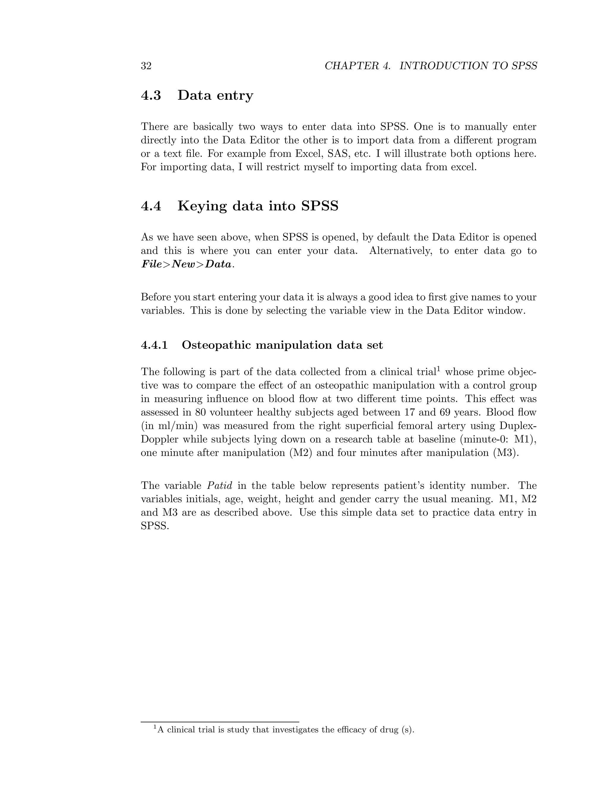
The following is part of the data collected from a clinical trial1 whose prime objec-
tive was to compare the effect of an osteopathic manipulation with a control group
in measuring influence on blood flow at two different time points. This effect was
assessed in 80 volunteer healthy subjects aged between 17 and 69 years. Blood flow
(in ml/min) was measured from the right superficial femoral artery using Duplex-
Doppler while subjects lying down on a research table at baseline (minute-0: M1),
one minute after manipulation (M2) and four minutes after manipulation (M3).
The variable Patid in the table below represents patient’s identity number. The
variables initials, age, weight, height and gender carry the usual meaning. M1, M2
and M3 are as described above. Use this simple data set to practice data entry in
SPSS.
1
A clinical trial is study that investigates the efficacy of drug (s).
4.4. KEYING DATA INTO SPSS 33
Table 4.1: Osteopathic Manipulation data set
Patid Initials Age Weight Height Gender M1 M2 M3
1 SJ 31 75 178 M 109.5 262.1 136.4
2 TG 30 69 178 M 103.2 145.7 121.3
3 SF 38 73 176 M 221.2 231.7 111.9
4 WD 24 78 179 M 230.0 281.3 196.2
5 VF 54 73 162 F 112.4 120.4 139.7
6 SM 64 75 168 M 226.8 369.4 247.1
7 DWM 61 65 160 F 103.7 84.9 109.5
8 GM 34 60 166 F 178.5 139.6 154.6
9 VM 38 64 165 F 103.7 132.4 107.1
10 DWF 47 63 167 M 150.6 158.8 110.4
11 BE 49 85 172 M 149.1 72.0 96.2
12 CV 55 91 177 M 193.5 286.1 245.5
13 CG 25 69 170 F 183.4 270.6 183.7
Exercise
Enter these data in your SPSS Data Editor window without labelling the variables.
If you enter the data in SPSS without first giving names to the variables, SPSS labels
the variables as var00001, var00002, etc. Do you see this?
Next try to give names to the variables. As described above, you can give names to
your variables via the variable view in the Data Editor window. Alternatively you
can double click the variable.
Now click on the first cell of the first column “Name” and type the name of the first
variable as indicated in Table 3. That is, Patid, and then move on to the second cell
and type the name of the second variable and so on.
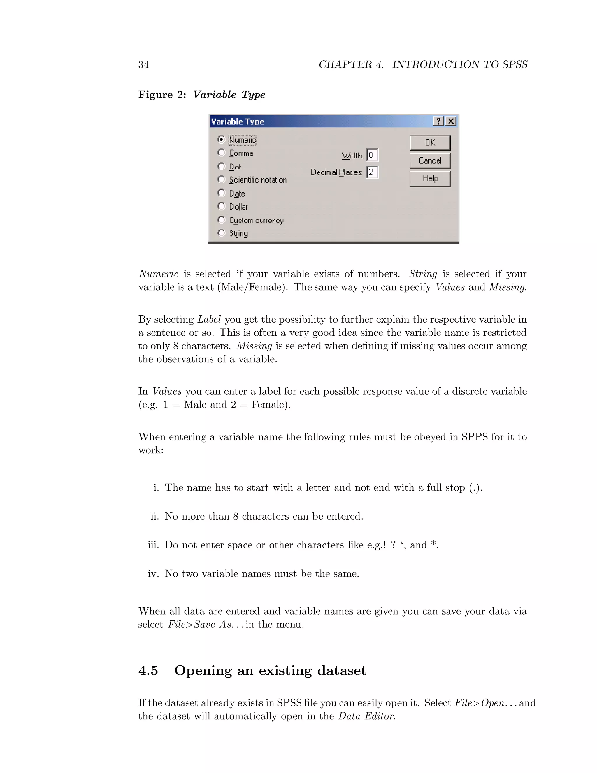
Under Type you define which type your variable is (numeric, string etc.). If you
place the marker in the Type cell, a button like the one in Figure 1 below appears.
Figure 1: Defining variables
This button indicates that you can click it and a window like the one below in Figure
2 will show:
34 CHAPTER 4. INTRODUCTION TO SPSS
Figure 2: Variable Type
Numeric is selected if your variable exists of numbers. String is selected if your
variable is a text (Male/Female). The same way you can specify Values and Missing.
By selecting Label you get the possibility to further explain the respective variable in
a sentence or so. This is often a very good idea since the variable name is restricted
to only 8 characters. Missing is selected when defining if missing values occur among
the observations of a variable.
In Values you can enter a label for each possible response value of a discrete variable
(e.g. 1 = Male and 2 = Female).
When entering a variable name the following rules must be obeyed in SPPS for it to
work:
i. The name has to start with a letter and not end with a full stop (.).
ii. No more than 8 characters can be entered.
iii. Do not enter space or other characters like e.g.! ? ‘, and *.
iv. No two variable names must be the same.
When all data are entered and variable names are given you can save your data via
select File>Save As. . . in the menu.
4.5 Opening an existing dataset
If the dataset already exists in SPSS file you can easily open it. Select File>Open. . . and
the dataset will automatically open in the Data Editor.
4.6. IMPORTING DATA 35
4.6 Importing data
Sometimes the data are available in a different format than an SPSS data file. E.g.
the data might be available as an Excel, SAS, or text file. As already mentioned we
describe how to import data from excel.
Importing data from Excel
If you want to use data from an Excel file in SPSS there are two ways to import the
data.
i. One is to simply mark all the data in the Excel window (excluding the variable
names) you want to enter into SPSS. Then copy and past them into the SPSS
data window. The disadvantage by using this method is that the variable
names cannot be included meaning that you will have to enter these manually
after pasting the data.
ii. The other option (where the variable names are automatically entered) is to
do the following:
• Open SPSS, select File> Open>Data. Choose the drive where the data are
stored and then double click on the file you want to open or mark the file and
click on the open icon on the open file menu.
Under Files of type you select Excel, press ‘Open’, and the data now appear
in the Data Editor in SPSS.
4.7 Exporting data
Exporting data from SPSS to a different program is done by selecting File Save
As. . . Under Save as type you select the format you want the data to be available in
e.g. Excel.
4.8 ANOVA for one-way classification in SPSS
Let us now see how we can use SPSS to perform analysis of variance for one way
classification. I will use the machine data set discussed in Section 5.3.4 to illustrate
the construction of the analysis of variance table. As described above, getting out-
puts in SPSS is simple. Assuming that you have already entered the data, what you
need to do next is to analyze the data by following the root below:
Analyze>Compare Means>One-Way ANOVA
If you click on the last option (One-Way ANOVA) you will see a window like the
one below:
36 CHAPTER 4. INTRODUCTION TO SPSS
The only dependent variable in this example is “volume” and the factor is “machine”.
You can also include descriptive statistics in your outputs by clicking on the ”Op-
tions” and then select descriptive.
Below is the SPSS ANOVA table for the machine data set.
SPSS ANOVA table-Machine data
Source of Sum of df Mean Square F Sig.
Variation Squares
Between Groups 0.152 3 5.072E-02 0.834 0.500
Within Groups 0.729 12 6.078E-02
Total 0.882 15
From the above ANOVA table we see that, the results presented in SPSS are approx-
imated to three decimal places. By default, SPSS, like any other software package
gives the p-value (s) of the test (s)-indicated as Sig. in the last column of the table.
The p-value indicates “how much evidence against the null hypothesis” has been
observed in the outcomes of the experiment. Based on the given p-value (> 0.5) we
do not reject the null hypothesis (remember we are testing the hypotheses at 0.05
level of significance), the conclusion we reached by comparing the F calculated value
(0.83) and the critical F-value (3.49) from the table. For comparison purposes of the
two ANOVA tables-the one we obtained before through mathematical calculations
and the one from SPSS above, I reproduce below the ANOVA table obtained by
mathematical computations. Are they similar?
Source of variation DF SS MS F- ratio
Between treatment 3 0.152145 0.051 0.83
Within treatment 12 0.729355 0.061
Total 15 0.881500
Exercise (optional)
Use the Pea section data set to perform analysis of variance for one way classification
4.8. ANOVA FOR ONE-WAY CLASSIFICATION IN SPSS 37
with equal replication. Compare your ANOVA table with the one obtained through
mathematical computations.
Note: The above two examples-the machine and pea section data sets illustrates
respectively what is termed as unbalanced and balanced data. Unbalanced in the
first case in the sense that there are unequal numbers of replications of machines
and balanced in the second case in the sense that the various sugar types are all
replicated equal number of times (10 times).
38 CHAPTER 4. INTRODUCTION TO SPSS
Chapter 5
Completely Randomized Design
5.1 Introduction
When the experimental units are assumed to be fairly uniform or homogeneous,
that is, no sources of variations other than the treatments are expected, grouping
them (applying error/local control principle) will be pointless in the sense that very
little (in terms of precision) may be gained. Thus, the simplest experimental design,
which incorporates only the first two principles (randomisation and replication) of
experimental designs, is the completely randomized design or CRD.
CRD is a design in which the treatments are assigned completely at random to the
experimental units, or vice-versa. Since we assume that there are no other sources of
variations in the experiment except the treatments under investigation, then CRD
imposes no restrictions, such as blocking on the allocation of the treatments to the
experimental units.
5.2 Layout
Suppose that we have t treatments under investigation and that the ithtreatment is
to be replicated ri times, i =1, 2, . . . , t. For an experiment with t treatments each
one replicated ri times, the total number of experimental units N =
t
i=1
ri. When
ri = r, that is, the case of equal replication, N=rt.
Definition: layout refers to the placement of treatment to the experimental units
subject to conditions of the design. Randomisation in CRD can be carried out by
using a random number table or any other probabilistic procedures.
Example
Suppose there are three treatments to be compared in a CRD. Suppose further
that the treatments are replicated 4, 3 and 5 times respectively. Thus, a total of
39
40 CHAPTER 5. COMPLETELY RANDOMIZED DESIGN
N =
t
i=1
ri=4 + 3 +5=12 experimental units. One possible layout of this experiment
is as follows:
T2
1
T1
2
T2
3
T3
4
T3
5
T1
6
T3
7
T1
8
T1
9
T3
10
T2
11
T3
12
5.3 Statistical analysis
The analysis of CRD is the same as that of one way classification. Let Yij be the
yield on the jthplot receiving treatment i. Thus, the model is:
Yij = µ + ti + eij, i=1, 2, . . . , t; j=1, 2, . . . r
Where:
µ is the grand mean (average) yield over all the N plots,
ti is the ith treatment effect
eij is the experimental error
Sums of squares are computed in the same way we discussed in one way classification.
5.3.1 Statistical hypotheses
The statistical hypotheses of interest as we stated before are:
Ho : µ1 = µ2 = ... = µt That is, the µi are all equal
H1 : µi = µj for at least one i = j. That is, the µi are not all equal.
Or simply
Ho :There is no variation among the treatments
H1 :Variation exists
5.4. ADVANTAGES AND DISADVANTAGES OF CRD 41
Table 5.1: ANOVA table
Source of Variation DF SS MS F-ratio
Treatments t-1 SSA SSA
t−1 = MSA MSA
MSE
Error N − t SSE SSE
N−t = MSE
Total N-1 SST
5.3.2 Test procedure
At level of significanceα, if F = MSA
MSE > Fα, [(t − 1) , (N − t)] then there is evidence
for no significance variation, i.e. we reject the null hypothesis. Otherwise, e do not
reject.
5.4 Advantages and disadvantages of CRD
5.4.1 Advantages
• Useful in small preliminary experiments and also in certain types of animal or
laboratory experiments where the experimental units are homogeneous.
• Flexibility in the number of treatments and the number of their replications.
• Provides maximum number of d.f. for the estimation of experimental error-
The precision of small experiment increases with error d.f.
5.4.2 Disadvantages
• Its use is restricted to those cases in which homogeneous experimental units
are available- local control not utilised. Thus, presence of entire variation may
inflate the experimental error.
• Rarely used in field experiments because the plots are not homogeneous.
5.5 Example
A sample of plant material is thoroughly mixed and 15 aliquots taken from it for
determination of potassium contents. 3 laboratory methods (I, II, and III) are em-
ployed. “I” being the one generally used. 5 aliquots are analysed by each method,
giving the following results (µg/ml).
I 1.83 1.81 1.84 1.83 1.79
Method II 1.85 1.82 1.88 1.86 1.84
III 1.80 1.84 1.80 1.82 1.79
Examine whether methods II and III give results comparable to those of method I.
Use α = 0.05
42 CHAPTER 5. COMPLETELY RANDOMIZED DESIGN
Calculations
The statistical model for this problem is Yij = µ + ti + eij. Here, i=1, 2, 3, j=1,2,
3, 4, 5.
Grand total, G =
3
i=1
5
j=1
Yij=1.83+1.81+. . . +1.79=27.4
Total number of observations, N =
k
i=1
ni =
3
i=1
ni = n1 + n2 + n3=5+5+5=15. In
the particular situation at hand (equal replication), N =rt =5×3=15
Correction factor, C.F=
3
i=1
5
j=1
Yij
2
rt = (27.4)2
15 = 750.76
15 =50.0507
Total sum of squared observations or uncorrected total sum of squares
3
i=1
5
j=1
Y 2
ij = (1.83)2
+ (1.81)2
+ ... + (1.79)2
= 50.0602
Total SS (SST) =
3
i=1
5
j=1
Y 2
ij − G2
rt =50.0602-50.0507=0.0095
=0.0095
Treatment (Method) totals: I=9.10, II=9.25, III=9.05
Treatment SS (SSTr) =1
r
k
i=1
Y 2
i − G2
rt , Yi =
r
j=1
Yij
=
1
5
(9.10)2
+ (9.25)2
+ (9.05)2
− 50.0507
=50.055-50.0507
=0.0043
Error SS (SSE) =SST-SSTr
=0.0095-0.0043
=0.0052
Table 5.2: ANOVA table
Source of Variation DF SS MS F-ratio
Between treatments 2 0.0043 0.00215 4.9654
Error (within treatments) 12 0.0052 0.00043
Total 14 0.0095
5.5. EXAMPLE 43
F0.05, 2, 12 = 3.89
Statistical hypothesis
Ho : µ1 = µ2 = µ3That is, the µi are all equal
H1 : µi = µjfor at least one i = j. That is, the µi are not all equal
Or
Ho: Methods do not differ
H1: Methods differ
Decision
Since the F calculated value (4.9654)> the critical F-value (3.89) at 0.05 level of
significance, we reject the null hypothesis and thus conclude that the laboratory
results depends on the method of analysis. That is, there exist significance variations
among the three laboratory methods.
To examine whether methods II and III give results comparable to those of method
I, we need to carry out further analysis using the t-test (LSD) as follows:
Let the mean of method I be denoted by ¯Y1., of method II by ¯Y2.and that of method
III by ¯Y3.
Thus, ¯Y1. = 9.10
5 = 1.82, ¯Y2. = 9.25
5 = 1.85, ¯Y3. = 9.05
5 = 1.81
Statistical Hypotheses
Here we need to test the hypotheses:
H02 : µ1 = µ3 vs. H12 : µ1 = µ3
H03 : µ1 = µ3 vs. H13 : µ1 = µ3
Test procedure
Reject: H02 if
| ¯Y2. − ¯Y1.| > LSD = s 2
r × tN−t,α/2
and H03 if | ¯Y3. − ¯Y1.| > LSD = s 2
r × tN−t,α/2
Exercises
1. Complete the test.
2. Eight varieties, A − H, of black currant cuttings are planted in square plots in a
nursery, each plot containing the same number of cuttings. Four plots of each variety
are planted, A and the shoot length made in the first growing season measured.
44 CHAPTER 5. COMPLETELY RANDOMIZED DESIGN
The plot totals are:
A: 46 29 39 35 E: 16 37 24 30
B: 37 31 28 44 F: 41 28 38 29
C: 38 50 32 36 G: 56 48 44 44
D: 34 19 29 41 H: 23 31 29 37
B and C are standard varieties; assess the remaining six for vigour in comparison
with B and C. Use α = 0.05
Chapter 6
Randomised Block Design
6.1 Introduction
CRD discussed in Chapter 3 will seldom be used if the experimental units are not
alike. Hence, when experimental units may be meaningfully grouped, e.g., by
area of field, device, hospital, salesmen, etc, clearly a completely randomised design
(CRD) will be insufficient. In this situation an alternative strategy for assigning
treatments to the experimental units, which takes advantage of the grouping, may
be used. The alternative strategy that we are going to discuss is what we call the
randomised block design or Randomised Complete Block Design (RCBD).
In the randomised block design:
• The groups are called blocks
• Each treatment appears the same number of times in each block; hence the
term complete block design
• The simplest case is that where each treatment appears exactly once in each
block. Here, because the number of replicates=number of experimental
units for each treatment,
we therefore have: number of replicates=number of blocks=r
• Blocks are often called replicates for this reason
• To set up such randomised block design the following steps are involved:
(i) Divide the units into r more homogeneous groups commonly known as blocks.
(ii) Assign the treatments at random to the experimental units within each block.
This randomisation has to be done afresh for each block.
Hence, the term randomised block design
45
46 CHAPTER 6. RANDOMISED BLOCK DESIGN
Motivation: experimental units within blocks are alike as possible, so observed
differences among them should be mainly attributed to the treatments. To ensure
this interpretation holds, in the conduct of the experiment, all experimental units
within a block should be treated as uniform as possible.
Intuitively speaking, randomised block design is an improvement over the CRD.
In the RBD the principle of local control can be applied along with the other two
principles of experimental design (randomisation and replication).
Number of experimental units (N )
Suppose we want to compare the effects of t treatments, each treatment being repli-
cated an equal number of times, say r times. Then we need N =rt experimental
units.
6.2 Layout
To illustrate the layout of an RBD, consider 4 treatments, each replicated 3 times.
So we need N =rt= 3×x4=12 experimental units which are grouped into 3 blocks
of 4 units.
Suppose the blocks formed after grouping the experimental units are labelled as 1,
2, and 3. To ensure randomness in every process involved in the experiment we
select the block to start with in allocating the treatments to the experimental units
at random. Assume the blocks are selected in the order 3, 1, 2. Thus, we start with
the third block and assign the 4 treatments at random to it. As we have discussed,
to assign the treatments, we may use any probabilistic procedure.
Permutations is one of the probabilistic procedures that may be used to allocate
treatments to experimental units. Suppose one of the permutations of the digits 1
to 4 for the treatment is 4, 1, 3, 2. Therefore we allocate treatment 4 in the first
unit of block 3, treatment 1 in the second unit of block 3, up to treatment 2 in the
fourth unit of block 3. That is, we have the following layout for block 3 (first selected
block).
T4 T1 T3 T2
Repeating the same procedure, suppose we select the permutations 3, 4, 2, 1 for
block 1 and 2, 3, 4, 1 for block 2, finally get the following complete layout.
6.3. STATISTICAL ANALYSIS 47
Block 1 T3 T4 T2 T1
Block 2 T2 T3 T4 T1
Block 3 T4 T1 T3 T2
6.3 Statistical analysis
The analysis of the design is the same as that of two-way classified data with one ob-
servation per cell-experimental unit- (without replication) we discussed in Section
5.5.
We use the same model we have discussed,
Yij = µ + ti + bj + eij, i=1, 2, . . ., t, j=1, 2, . . ., r
In words:
Observation of the ith treatment from the jth block =general mean +ith treatment
effect + jth block effect + experimental error component
RECAP: we partition the total sum of squares into different components:
Total SS=Treatment SS + Block SS + Error SS
6.3.1 Statistical hypotheses
The hypotheses of interest are:
HO1 : t1 = t2 = ... = tk
Ho2 : b1 = b2 = ... = bk
Against their alternative that tis, bjs are not all equal.
ANOVA table
Source of variation DF SS MS F-ratio
Blocks r-1 SSB SSB
r−1 = MSB MSB
MSE = FB
Treatment t-1 SSTr
SSTr
t−1 = MSTr
MSTr
MSE = FT r
Error (r-1)(t-1) SSE SSE
(r−1)(t−1) = MSE
Total N-1 SST
6.3.2 Test procedure
The calculated F-values for treatments and blocks (FBand FTr) are compared with
the tabulated (critical) F-values at (t-1) and (r-1)(t-1) and (r-1) and (r-1)(t-1) de-
grees of freedom respectively.
48 CHAPTER 6. RANDOMISED BLOCK DESIGN
In symbols
Fα, [(t − 1), (r − 1)(t − 1)] and Fα, [(r − 1), (r − 1)(t − 1)]
Thus, if FB>Fα, [(r − 1), (r − 1)(t − 1)] we reject the null hypothesis, otherwise we
do not reject. Also if FTr>Fα, [(t − 1), (r − 1)(t − 1)] we reject the null hypothesis,
otherwise we do not reject.
6.4 Advantages and disadvantages of RBD
6.4.1 Advantages
• Greater precision
• Increased scope of inference is possible because more experimental conditions
may be included
6.4.2 Disadvantages
• Large number of treatments increases the block size; as a result the block may
loose homogeneity leading to large experimental error.
• Any missing observation in a unit in a block will lead to either:
(i) discard the whole block
(ii) estimate the missing value from the unit by special missing plot technique.
6.5 Example
The following data are yields in bushels/acre from an agricultural experiment set out
in a randomised complete clock design. The experiment was designed to investigate
the differences in yield for seven hybrid varieties of wheat, labelled A-G here. A field
was divided into 5 blocks, each containing 7 plots. In each plot, the seven plots were
assigned at random to be planted with the seven varieties, one plot for each variety.
A yield was recorded for each plot. Examine whether varieties affect the yield. Use
α=0.05.
Variety
Block A B C D E F G Total
I 10 9 11 15 10 12 11 78
II 11 10 12 12 10 11 12 78
III 12 13 10 14 15 13 13 90
IV 14 15 13 17 14 16 15 104
V 13 14 16 19 17 15 18 112
Total 60 61 62 77 66 67 69 G=462
6.5. EXAMPLE 49
We assume that the measurements are approximately normally distributed, with the
same variance σ2.
Calculations
Total number of experimental observation (N) = r × t= 7×5=35
Grand total (G) =
t
i=1
r
j=1
yij=10 + 9 +. . . + 15 + 18=462
Correction factor (C.F) =G2
N = (462)2
35 =6098.4
Uncorrected total sum of squares
t
i=1
r
j=1
y2
ij=102 +92 +. . . + 152 + 182 =6314.0
Total sum of squares (SST) =
t
i=1
r
j=1
y2
ij-C.F= 6314.0 - 6098.4=215.6
Treatment (variety) sum of squares (SSTr) = 1
r
t
i=1
Y 2
i -C.F
=1
5(602 + ... + 692)-C.F
=6140.0-6098.4
=41.6
Block sum of squares (SSB) = 1
t
r
j=1
Y 2
j -C.F
=1
7(782 + ... + 1122)-C.F
=6232.6-6098.4
=134.2
Error sum of squares (SSE) =Total SS-Treatment SS-Block SS
= 215.6-134.2-41.6=39.8
Treatment (variety) mean squares (MSTr) = SSTr
t−1 = 41.6
6 =6.93
Block mean squares (MSB) = SSB
r−1 = 134.2
4 =33.54
Error mean squares (MSE) = SSE
(t−1)(r−1) = 39.8
24 =1.66.
Finally, we estimate the F-values. For block the F-calculated value is
50 CHAPTER 6. RANDOMISED BLOCK DESIGN
=MSB
MSE = 33.54
1.66 =20.21 and
for treatments the F-calculated value is MSTr
MSE = 6.93
1.66=4.18
We summarize the calculations in an ANOVA table as follows:
ANOVA Table
Source of variation D.F SS MS F-ratio
Blocks 4 134.2 33.54 20.21
Treatments 6 41.6 6.93 4.18
Error 24 39.8 1.66
Total 34 215.6
To perform the hypothesis test for differences among the treatment means, we com-
pare the F calculated values to the appropriate value from the F table. For level of
significance α=0.05, we have
F0.05;6,24 = 2.51. F-calculated (= 4.18)> F0.05;6,24 = 2.51.
Therefore, we reject H0. There is evidence in these data to suggest that there are
differences in mean yields among the varieties.
To test the hypothesis on block differences, we find F0.05,4,24=2.78. We have 20.21>2.87,
thus, we also reject H0. There is strong evidence in these data to suggest differ-
ences in mean yield across blocks at the 5% level of significance.
In SAS
data hybrid;
input Block $ Variety $ Yield @@;
cards;
I A 10 I B 9 I C 11 I D 15 I E 10 I F 12 I G 11
II A 11 II B 10 II C 12 II D 12 II E 10 II F 11 II G 12
III A 12 III B 13 III C 10 III D 14 III E 15 III F 13 III G 13
IV A 14 IV B 15 IV C 13 IV D 17 IV E 14 IV F 16 IV G 15
V A 13 V B 14 V C 16 V D 19 V E 17 V F 15 V G 18
;
run;
proc print;run;
proc anova;
class Block Variety ;
model Yield=Block Variety;
run;quit;
The SAS System
Obs Block Variety Yield
1 I A 10
6.5. EXAMPLE 51
2 I B 9
3 I C 11
4 I D 15
5 I E 10
6 I F 12
7 I G 11
8 II A 11
9 II B 10
10 II C 12
11 II D 12
12 II E 10
13 II F 11
14 II G 12
15 III A 12
16 III B 13
17 III C 10
18 III D 14
19 III E 15
20 III F 13
21 III G 13
22 IV A 14
23 IV B 15
24 IV C 13
25 IV D 17
26 IV E 14
27 IV F 16
28 IV G 15
29 V A 13
30 V B 14
31 V C 16
32 V D 19
33 V E 17
34 V F 15
35 V G 18
Class Level Information
Class Levels Values
Block 5 I II III IV V
Variety 7 A B C D E F G
Number of observations 35
Dependent Variable: Yield
Sum of
Source DF Squares Mean Square F Value Pr > F
Model 10 175.7714286 17.5771429 10.59 <.0001
Error 24 39.8285714 1.6595238
Corrected Total 34 215.6000000
R-Square Coeff Var Root MSE Yield Mean
0.815266 9.759281 1.288225 13.20000
52 CHAPTER 6. RANDOMISED BLOCK DESIGN
Source DF Anova SS Mean Square F Value Pr > F
Block 4 134.1714286 33.5428571 20.21 <.0001
Variety 6 41.6000000 6.9333333 4.18 0.0052
6.6 Reasons for blocking in RBD
Note from these results that the blocking served to explain much of the overall vari-
ation. To appreciate this further, suppose that we had not blocked the experiment,
but instead had just conducted the experiment according to a completely random-
ized design. Suppose that we ended up with the same data as in the experiment
above.
Under these conditions variety is the only classification factor for the plots, and we
would construct the following analysis of variance table for one way-classification as
discussed in the previous sections.
ANOVA Table
Source of variation DF SS MS F-ratio
Between treatments (varieties) 6 41.6 6.93 1.12
Within treatments (error) 28 174.0 6.21
Total 34 215.6
The test for differences in mean yield for the varieties (treatments) would be to
compare F=1.12 to F0.05,6,28=2.45. Note that we would thus not reject H0 of no
treatment differences at the 5% level of significance.
Concluding Remark
From the above example, it is immediately clear that if the different sources of
variation are not properly identified (e.g., due to erroneously accounting for the
experimental design), then invalid conclusions will be drawn.
The example discussed above clearly demonstrates the aspect of wrongly identify-
ing the experimental design. In the one-way classification experiment and analysis
presented above, there is no accounting for the variation in the data that is actually
attributable to a systematic source, position in the field (the factor used to block
the experiment). The one-way analysis has no choice but to attribute this variation
to experimental error; that is, it regards this variation as just part of the inherent
variation among experimental units that we cannot explain. The result is that the
Error SS in the one-way analysis contains both variation due to position in the field
(which is actually systematic variation) and inherent variation.
Here, note that 143.2+39.8=174.0 and 4+24=28.
This is the Error SS for the one-way classification analysis. Which actually may be
regarded as ignoring the blocks (because what we really did was to pretend that the
6.6. REASONS FOR BLOCKING IN RBD 53
blocks didn’t exist) and thus resulting into big MSE in which we could not reject the
H0. By blocking the experiment, and explicitly acknowledging position in the field
as a potential source of variation, MSE was sufficiently reduced so that we could
identify variety differences.
It can be learned from this example that:
• Blocking may be an effective means of explaining variation (increasing preci-
sion) so that differences among treatments that may really exist are more likely
to be detected.
• The data from an experiment set up according to a particular design should
be analysed according to the appropriate procedure for that design. The
above shows that if we set up the experiment according to a randomised com-
plete block design, but then analyse it as if it had been set up according to
a completely randomised design, erroneous inferences results, in this case,
failure to identify real treatment differences. Remember, the design of an
experiment dictates the analysis!!
Exercise
Four different plant densities A-D are included in an experiment on the growth of
lettuce. The experiment is laid out as a randomised block, and the same number of
plants is harvested from each plot, giving the weights (recorded) below. Examine
whether density appears to affect the yield. Use α = 0.01
54 CHAPTER 6. RANDOMISED BLOCK DESIGN
Block
Density I II III IV V VI
A 2.7 2.6 3.1 3.0 2.5 3.0
B 3.0 2.8 3.1 3.2 2.8 3.1
C 3.3 3.3 3.5 3.4 3.0 3.2
D 3.2 3.0 3.3 3.2 3.0 3.1
Chapter 7
Latin Square Design
7.1 Introduction
There are often situations where it may be necessary to account for two sources
of variation by blocking. If the number of treatments and levels of each blocking
factor is large, the size of the experiment may become unwieldy or resources may be
limited. Thus, in agricultural field experiments (and other situations), a particular
setup is often used that allows differences among treatments to be assessed with less
recourses.
The principle of local control was used in the RBD by grouping the units in one
way; i.e. according to blocks. The grouping can be carried one step forward and
we can group the units in two ways, each way corresponding to a known source of
variation among the units, and get the Latin Square Design (LSD). This design is
used with advantage in agricultural experiments where the fertility contours are not
always known. It has also been used successfully in industry and in the laboratory.
Latin square design is a design, which uses the principle of local control twice.
RBD removes one systematic source of variation in addition to treatments, but LSD
removes two such sources. Hence, LSD is a three-way classification.
In a field experiment if two probable fertility trends can be thought of, in directions
at right angles, both need to be made the basis of blocking. Thus when there is a
slope of the land being used, and also a climatic trend (e.g. effects of wind, rain) at
right angles to this, a randomised block cannot take out all the known variation.
7.2 Layout
In field experiments, the physical layout is that of a square with rows of plots. In
this set up the layout is such that every letter (A, B, C,. . . ) the set of treatments
occurs exactly once in each row and in each column. For four letters A, B, C, and
D the layout would be as shown below.
55
56 CHAPTER 7. LATIN SQUARE DESIGN
Column 1 2 3 4 5
1 E B A D C
2 C A D E B
Row 3 B E C A D
4 A D B C E
5 D C E B A
This type of setup would be useful when for example variability due to soil differences,
etc, arises in two directions. Each plot would constitute a single experimental unit.
This particular kind of setup with two blocking variables (rows and columns), in
which the numbers of rows, columns and treatments are the same, is known as a
Latin square.
Notation
Because the number of treatments, rows and columns are the same, the number
of replicates on each treatment is equal to the number of treatments, rows, and
columns. We will denote this as t. For given value of t, there may be several ways
to construct a Latin square. This is actually as mathematical exercise. Extensive
listings of ways to construct Latin squares for different values of t are often given in
texts on experimental design (see for example, Montgomery, 2001).
Selection of LSD
The totality of LSD’s obtained from a single LSD by permuting rows, columns and
treatments (letters) is called a transformation set.
e.g. A B C D fixed
B C D A
C D A B
D A B C
A B C D
C D A B
D A B C
B C D A
A k×k Latin Square with k letters A, B, C, . . . in the natural order occurring in the
first column is called a standard square (square in canonical form).
e.g. A B C D
B C D A
C D A B
D A B C
From a standard k × k Latin Square, we may obtain k! (k-1)! Different LSD’s by
permuting all the k columns and the (k-1) rows except the first row. Hence there
7.3. STATISTICAL ANALYSIS 57
are in all k! (k-1)! Different LSDs with the same standard square. Thus the total
number of different LSDs in a transformation set is k! (k-1)! times the number of
standard LSDs in the set. In order to give all k × k LSDs equal probability of being
selected, we select one LSD from all k × k LSDs and then randomise the columns
and rows, excluding the first row (if it is the fixed one).
Randomisation consists of choosing one of the possible designs for given t at random.
Then randomly assign the letters A, B, C, etc to the treatments of interest
7.2.1 Linear additive model
To write down a model, we need to be a bit careful with the notation. The key is
that, although we have three classifications (row, column and treatment) we do not
have t × t × t = t3 observations; rather we only have t × t = t2
The mathematical model will now be,
yijk = µ + ti + rj + ck + eijk
where:
yijk observation for the ith treatment appearing in row j, column k
µ is an overall mean
rj, ck represents the effects of the jth row and kth column
ti represents the effect of the treatment appearing at position, j,k
eijk error associated with the experimental unit appearing at position j,k
7.3 Statistical analysis
The analysis proceeds along the same lines as for RBD, but instead of the one sum
of squares for blocks; systematic variation is now taken out by two sums of squares,
which are always called Rows (SSR) and columns (SSC).
7.3.1 Calculation of sums of squares
To setup the analysis of variance we define Rjand Ck as the totals of all plots in the
jth row and kth column respectively in the layout, the sums of squares required are:
Total SS SST =
t
i=1
t
j=1
t
k=1
y2
ijk − G2
t2
Row SS (SSR)=1
t
t
j=1
R2
j − G2
t2
Column SS (SSC)=1
t
t
k=1
C2
k − G2
t2
58 CHAPTER 7. LATIN SQUARE DESIGN
Treatment SS (SSTr) = 1
t
t
i=1
T2
i − G2
t2
Error SS (SSE)= SST –(SSR+SSC+SSTr) or
SSE =SST – SSR –SSC -SSTr
The degrees of freedom for SSR, SSC, SSTr are each (t-1); for SST, (t2-1), and so
for SSE, (t2-1)-3 (t-1), reducing to (t-1)(t-2).
Table 7.1: Three way ANOVA table
Source of DF SS MS F-ratio
variation
Rows t-1 SSR SSR
t−1 = MSR MSR
MSE = FR
Columns t-1 SSC SSC
t−1 = MSC MSC
MSE = FC
Treatments t-1 SSTr SSTr
t−1 = MSTr
MSTr
MSE = FTr
Error (t-1)(t-2) SSE SSE
(t−1)(t−2) = MSE
Total t2-1 SST
7.4 Advantages and disadvantages of LSD
7.4.1 Advantages
• Eliminates from the error two major sources of variation. Hence LSD is an
improvement over RBD in controlling error by planned grouping just as the
RBD is an improvement over CRD.
• LSD is a 3-way incomplete layout since LSD considers treatments, rows, and
columns at the same number of levels t, we would need a complete three way
layout of t3 number of experimental units. However, since we are using t2
number of experimental units, then it is said to be a 3-way incomplete layout.
7.4.2 Disadvantages
• A serious limitation of the LSD is that the number of replicates must be the
same as the number of treatments, the larger the square the more is the repli-
cates, hence the bigger the blocks (columns and rows). Hence larger squares
(over 12×12 ) are seldom used in the sense that the squares does not remain
homogeneous. On the other hand, small squares provide only a few degrees of
freedom for the error. Preferable LSDs are form 5×5 to 8×8.
• The analysis depends heavily on the assumption that there are no interactions
present.
• Analysis becomes very difficult where there are missing observations.
7.5. EXAMPLE 59
7.5 Example
The following is a 5×5 Latin square for data taken from a manurial experiment with
sugarcane. The five treatments were as follows:
A: no manure
B: no inorganic manure
C, D and E: three levels of farm yard manure.
Column
Row I II III IV V
I A:52.5 E: 46.3 D:44.1 C:48.1 B:40.9
II D:44.2 B: 42.9 A:51.3 E:49.3 C:32.6
III B:49.1 A:47.3 C:38.1 D:41.0 E:47.2
IV C:43.2 D:42.5 E:67.2 B:55.1 A:45.3
V E: 47.0 C:43.2 B:46.7 A:46.0 D:43.2
Analyse the data to find out if there are any treatment effects. Use α = 0.05and
α = 0.01
Calculations
The statistical model for this problem is
yijk = µ + ti + rj + ck + eijk, i =1,2,. . . ,t;j=1,2,. . . t; k=1,2,. . . t
Since we have 5 rows, 5 columns, and 5 treatments (letters) appearing only once in
each row and in each column, hence the design is a Latin square (i.e. 5×5 Latin
square). So the model becomes,
yijk = µ + ti + rj + ck + eijk; i=1, 2, 3, 4, 5; j=1, 2, 3, 4, 5; k=1, 2, 3, 4, 5
The total number of experimental units (N) = t2= 5×5=25
The grand total (G) =
t
i=1
t
j=1
t
k=1
yijk
=
5
i=1
5
j=1
5
k=1
yijk=52.5+46.3+. . . +46.0+43.2= 1154.3
Correction factor (C.F) =
⎛
⎜
⎜
⎝
t
i=1
t
j=1
t
k=1
yijk
t
⎞
⎟
⎟
⎠
2
= G
t
2
or G2
t2
=
⎛
⎜
⎜
⎝
5
i=1
5
j=1
5
k=1
yijk
5
⎞
⎟
⎟
⎠
2
= 1154.3
52
2
= 1332408.49
25 =53296.3333
=53296.3333 (4.dec.places)
Total SS (SST) =
t
i=1
t
j=1
t
k=1
y2
ijk − G2
t2 (or C.F)
60 CHAPTER 7. LATIN SQUARE DESIGN
=
5
i=1
5
j=1
5
k=1
y2
ijk − G2
52 , but
5
i=1
5
j=1
5
k=1
y2
ijk = 54273.51
⇒SST= 54273.51-53296.3333=977.1767
SST= 977.1767
Row SS (SSR)=1
t
t
j=1
R2
j − G2
t2
=1
5
5
j=1
R2
j − G2
52
Row totals:
R1=52.5+46.3+44.1+48.1+40.9=231.9
R2=44.2+42.9+51.3+49.3+32.6=220.3
R3=49.1+47.3+38.1+41.0+47.2=222.7
R4=43.2+42.5+67.2+55.1+45.3=253.3
R5=47.0+43.2+46.7+46.0+43.2=226.1
⇒SSR=1
5 R2
1 + R2
2 + R2
3 + R2
4 + R2
5 − C.F
= 1
5 231.92 + 220.32 + 222.72 + 253.32 + 226.12 − 53296.3333
=1
5 (267187.09) − 53296.3333
=53437.4180-53296.3333=141.0847
Column SS (SSC) =1
t
t
k=1
C2
k − G2
t2
=1
5
5
k=1
C2
k − G2
52
Column totals:
C1=52.5+44.2+49.1+43.2+47.0=236.0
C2=46.3+42.9+47.3+42.5+43.2=222.2
C3=44.1+51.3+38.1+67.2+46.7=247.4
C4=48.1+49.3+41.0+55.1+46.0=239.5
C5=40.9+32.6+47.2+45.3+43.2=209.2
⇒SSC=1
5 C2
1 + C2
2 + C2
3 + C2
4 C2
5 − C.F
=1
5 236.02 + 222.22 + 247.42 + 239.52 + 209.22 − 53296.3333
=1
5 (267400.49) − 53296.3333
=53480.0980-53296.3333
=183.7647
7.5. EXAMPLE 61
Treatment SS (SSTr) =1
t
t
i=1
T2
i − G2
t2
=1
5
5
i=1
T2
i − G2
52
Treatment totals:
A=52.5+51.3+47.3+45.3+46.0=242.4
B=40.9+42.9+49.1+55.1+46.7=234.7
C=48.1+32.6+38.1+43.2+43.2=205.2
D=44.1+44.2+41.0+42.5+43.2=215.0
E=46.3+49.3+47.2+67.2+47.0=257.0
⇒SSTr =1
5 T2
1 + T2
2 + T2
3 + T2
4 + T2
4 − C.F
=1
5 242.42 + 234.72 + 205.22 + 215.02 + 257.02 −53296.3333
=1
5 (268222.89) −53296.3333
=53644.5780-53296.3333
=348.2447
Error sum of squares (SSE)=SST-(SSR+SSC+SSTr)
=SST-SSR-SSC-SSTr
=977.1767-141.0847-183.7647-348.2447=304.0826
ANOVA Table
Source of DF SS MS F-ratio
variation
Rows 4 141.0847 35.2712 1.3919
Columns 4 183.7647 45.9412 1.8130
Treatments 4 348.2447 87.0612 3.4357
Error 12 304.0826 25.3402
Total 24 977.1767
F0.05, 4,12=3.26, F0.01, 4,12=5.41
Hypotheses:
H01: No treatment effects
H02: No row effects
H03: No column effects
Against their alternatives
Test procedure
The hypothesis of no treatment effect is not rejected at the 1% (0.01) level of
significance since the calculated F value (3.4357) is less than the tabulated F value
(5.41), but rejected at the 5% (0.05) level of significance since the calculated F value
(3.4357) is greater than the tabulated F value (3.26). Thus, the amount of sugarcane
62 CHAPTER 7. LATIN SQUARE DESIGN
produced will depend upon which type of manure is used. Or manures affect yields.
In SAS
data lsd;
input Block $ Column $ Manure $ Yield @@;
cards;
I I A 52.5 I II E 46.3 I III D 44.1 I IV C 48.1 I V B 40.9
II I D 44.2 II II B 42.9 II III A 51.3 II IV E 49.3 II V C 32.6
III I B 49.1 III II A 47.3 III III C 38.1 III IV D 41.0 III V E 47.2
IV I C 43.2 IV II D 42.5 IV III E 67.2 IV IV B 55.1 IV V A 45.3
V I E 47.0 V II C 43.2 V III B 46.7 V IV A 46.0 V V D 43.2
;
proc print;run;
proc anova;
class Block Column Manure ;
model Yield=Block Column Manure;
run;quit;
Obs Block Column Manure Yield
1 I I A 52.5
2 I II E 46.3
3 I III D 44.1
4 I IV C 48.1
5 I V B 40.9
6 II I D 44.2
7 II II B 42.9
8 II III A 51.3
9 II IV E 49.3
10 II V C 32.6
11 III I B 49.1
12 III II A 47.3
13 III III C 38.1
14 III IV D 41.0
15 III V E 47.2
16 IV I C 43.2
17 IV II D 42.5
18 IV III E 67.2
19 IV IV B 55.1
20 IV V A 45.3
21 V I E 47.0
22 V II C 43.2
23 V III B 46.7
24 V IV A 46.0
25 V V D 43.2
Dependent Variable: Yield
Sum of
Source DF Squares MS F-Value Pr > F
Model 12 673.0752 56.0896 2.21 0.0916
Error 12 304.0952 25.3413
Corrected Total 24 977.1704
7.5. EXAMPLE 63
R-Square Coeff Var Root MSE Yield Mean
0.688800 10.90274 5.034011 46.17200
Source DF Anova SS MS F Value Pr > F
Block 4 141.0784 35.2696 1.39 0.2948
Column 4 183.7584 45.9396 1.81 0.1912
Manure 4 348.2384 87.0596 3.44 0.0431
Exercises
1. Using the ANOVA table above, examine whether there are any significance dif-
ferences between the rows and between the columns at 1% level of significance.
2. A supermarket organisation buys in a particular foodstuff from four suppliers
A, B, C, D and subjects samples of this to regular tasting tests by expert panels.
Various characteristics are scored, and the total score for the product is recorded.
Four tasters a, b, c, d at four sessions obtained the results below. Analyse and
comment on these. Use α = 0.05
Taster
a b c d
1 A: 21 B: 17 C: 18 D: 20
Session 2 B: 20 D: 22 A: 23 C: 19
3 C: 20 A: 24 D: 22 B: 19
4 D: 22 C: 21 B: 22 A: 26
3. Five different aptitude tests, A-E are applied on five successive days to five
different students who are considered comparable in intelligence. None of them has
previously attempted tests of this type, and so it is required to remove any possible
differences between days, which could be attributed to a learning effect. Investigate
the validity of the claim that the tests measure the same qualities, and also examine
differences between students and between days.
Scores Day 1 2 3 4 5 Student Totals for
totals tests
1 E: 56 B: 62 A: 65 D: 59 C: 76 318 A: 331
2 C: 74 A: 65 D: 60 E: 61 B: 70 330 B: 332
Student 3 B: 63 E: 59 C: 80 A: 66 D: 64 332 C: 393
4 A: 64 D: 63 B: 67 C: 81 E: 64 339 D: 310
5 D: 64 C: 82 E: 64 B: 70 A: 71 351 E: 304
Day totals 321 331 336 337 345 1670 1670
64 CHAPTER 7. LATIN SQUARE DESIGN
Chapter 8
Factorial Experiments
8.1 Introduction
In the previous discussions we considered factor(s) at different levels separately and
examined their significance. In practice, sometimes the interest is to evaluate the
effects of a combination of more than one factor each at two or more levels.
Experiments where the effects of more than one factor, say variety, manure, etc., each
at two or more levels, are considered together are called factorial experiments,
while experiments with one factor at varying levels, say only variety or manure, may
be called simple experiments.
It is customary to represent the factors by small letters a, b, c, etc. A treatment is
then determined by a combination of different levels of factor aibjck etc. For exam-
ple, if we have two factors a and b each at two levels, zero and one (i.e. i = 0, l, j
= 0, 1) then the four treatment combinations are aobo, aob1, a1bo and a1b1. The
comparisons among the treatment combinations are called the effects, which are
represented by capital, letters A, B, C, D etc.
When each treatment combination is used the same number of times, the factor-
ial experiment is known as complete factorial experiment. The experiment is
described as pn factorial experiment when there are n factors and each factor is con-
sidered at p levels. For example a three factors experiment with each factor having
two levels, then we say we have a 23 factorial experiment. In this course we shall
consider only the simplest cases, i.e. cases of n factors each at 2(or 3) levels or
what are known as 2n(3n) experiments, where n is any positive integer greater than
or equal to 2. Generalisation to any complex situations (factorial experiments) is
straightforward.
65
66 CHAPTER 8. FACTORIAL EXPERIMENTS
8.2 Main effects and interaction effects
The effects in a factorial experiment are composed of main effects and interaction
effects.
A main effect of a factor is defined as a measure of the average change in effect
produced by changing the levels of the factor. It is measured independently of other
factors.
Factors are said to interact when they are not independent. But “interaction”
in a factorial experiment is a measure of the extent to which the effect of changing
the levels of one or more factors depends on the levels of the other factors.
Interactions between two factors are referred to as first order interaction, those
concerning three factors are referred to as second order interaction and so on.
8.3 The 22
factorial experiments
Let the symbols aibj (i=o, l, j=o,l) represent both the treatment combination and
yields from all experimental units or plots.
Effect of factor a at level b0 of factor b = a1b0 – a0b0.
Effect of factor a at level b1 of factor b = a1b1 – a0b1.
Therefore, the main effect of factor a = average change produced by varying the
levels of factor a.
= 1
2 [(a1bo − aobo) + (a1b1 − aob1)]
= 1
2 [b0 (a1 − ao) + b1 (a1 − ao)]
= 1
2 [(a1 − ao) (bo + b1)]
Therefore, the main effect of factor a = 1
2 (a1 − ao) (bo + b1) = A
Similarly the main effect of factor b.
Effect of factor b at level a0 of factor a
= a0b1-a0b0
Effect of factor b at level a1, of factor a
= a1b1-a1b0
8.3. THE 22 FACTORIAL EXPERIMENTS 67
Therefore, the main effect of factor b
= 1
2 [(aob1 − aobo) + (a1b1 − a1bo)]
= 1
2 [(b1 − b0) a0 + (b1 − b0) a1]
= 1
2 [(b1 − b0) (a0 + a1)]
= 1
2 (b1 − b0) (a1 + a0) = B
If the two factors “a” and “b” were acting independently the effect of factor a at
level b0 and the effect of factor a at level b1 or the effect of factor b at level a0 and
the effect of factor b at level a1 should be equal, but in general they will be different.
This difference is a measure of the extent to which the factors interact. Hence A×B,
the interaction between two factors “a” and “b” each at 2 levels, zero and one is
given by
A × B =
1
2
[(a1b1 − a0b1) − (a1b0 − a0b0)]
A × B =
1
2
(a1 − a0) (b1 − b0)
It is clear from this relation that interaction between factors “a” and “b” i.e. A×B
is the same as that between “b” and “a” i.e. B×A.
The overall mean is represented by M
i.e. M = 1
4 [a0b0 + a0b1 + a1b0 + a1b1]
= 1
4 [a0(b0 + b1) + a1(b0 + b1)]
=1
4 [(a0 + a1)(b0 + b1)]
= 1
4 (a1 + a0) (b1 + b0)
Replacing the symbols a0 and b0 by 1 and the symbols a1 and b1 by simple aand b
respectively, the preceding comparisons may be expressed by
A = 1
2 (a − 1) (b + 1)
B = 1
2 (a + 1) (b − 1)
AB = 1
2 (a − 1) (b − 1)
68 CHAPTER 8. FACTORIAL EXPERIMENTS
M = 1
4 (a + 1) (b + 1)
Expanding say A, A = 1
2 [ab + a − b − 1]
= 1
2 [ab − b + a − 1]
Then, these effects can be conveniently written in a table of plus and minus signs as
shown below:
Effect Treatment Combination Divisor
(1) a b ab
M + + + + 4
A - + - + 2
B - - + + 2
AB + - - + 2
Note: It should be noted that the effects A, B, and AB are three mutually orthogonal
contrasts of the yields of the 4 treatments each based on 1 d.f. i.e. The sum of
products of the corresponding coefficients of the contrasts say A and AB is equal to
zero.
8.4 The 23
factorial experiments
In this case we consider 3 factors a, b, and c each at 2 levels. Hence we get 8 different
treatment combinations, which are listed below.
a0b0c0, a1b0c0, a0b1c0, a0b0c1, a1b1c0, a1b0c1,a0b1c1, a1b1c1 or
(1), a, b, c, ab, ac, bc, abc
The main effects and interactions as defined before can be represented by the fol-
lowing relations:
A = 1
4 (a − 1) (b + 1) (c + 1)
B = 1
4 (a + 1) (b − 1) (c + 1)
C = 1
4 (a + 1) (b + 1) (c − 1)
AB = 1
4 (a − 1) (b − 1) (c + 1)
AC =1
4 (a − 1) (b + 1) (c − 1)
BC = 1
4 (a + 1) (b − 1) (c − 1)
8.5. SUM OF SQUARES DUE TO FACTORIAL EFFECTS 69
ABC = 1
4 (a − 1) (b − 1) (c − 1)
The overall mean in this case is written as
M = 1
8 (a + 1) (b + 1) (c + 1)
The divisor (8) is due to the fact hat we have 8 different treatment combinations (as
listed above) to average out.
Expanding A we have,
A = 1
4 [− (1) + (a) − (b) + (ab) − (c) + (ac) − (bc) + (abc)]
Similarly, expanding B we have
B = 1
4 [− (1) − (a) + (b) + (ab) − (c) − (ac) + (bc) + (abc)]
The expression above can also be summarized by the following plus and minus signs
table.
Effect Treatment Combination Divisor
(1) a b ab c ac bc abc
M + + + + + + + + 8
A - + - + - + - + 4
B - - + + - - + + 4
C - - - - + + + + 4
AB + - - + + - - + 4
AC + - + - - + - + 4
BC + + - - - - + + 4
ABC - + + - + - - + 4
The above table can be extended to include up to n factors all at two levels by
corresponding the expression:
1
2n−1 (a ± 1) (b ± 1) (c ± 1)
Where a minus sign appears in any factor on right if the corresponding letter is
on the left or give to each of the treatment combination a plus sign where the
corresponding factor is at the second level and a minus sign where it is at the first
level.
8.5 Sum of squares due to factorial effects
To conduct the tests of significance using the analysis of variance technique, we need
to estimate the sum of squares. In factorial experiments the basic sum of squares
70 CHAPTER 8. FACTORIAL EXPERIMENTS
are computed in the usual way with the addition that the treatment sum of squares
is further partitioned into component parts of main effects and interaction.
The design structure may be CRD, RBD or LSD but it is the treatments that have
a factorial structure.
To compute the sum of squares let us consider a 22 factorial experiment, which has
been carried out in an RBD with r replications or blocks. The statistical model as
we discussed before would be:
yij = µ + ti + bj + eij
The block SS, Treatment SS and error SS are computed in the usual way. However,
since our interest is in the main effect and interaction effects. We obtain their SS as
follows.
Define the effect totals by []
i.e. [A] = − [1] + [a] − [b] + [ab]
Then the SS due to any main effect or the interaction effect is obtained by multiplying
the square of the effect total by the reciprocal of 4r, where r is the common replication
number. Thus.
SS due to main effect of A = [A]2
4r with d.f. = 1;
SS due to main effect of B = [B]2
4r with d.f. = 1;
SS due to interaction effect of AB = [AB]2
4r with d.f. = 1;
With this model, the analysis of variance table would be as follows:
Table 8.1: ANOVA table for a 22 experiment in r randomised blocks
Source of Variation d.f. S.S. M.S. F-ratio
Blocks r - 1 SS (Blocks) MS (Blocks) MS(Blocks)
Treatments
Main effect A 1 [A]2
4r MSA MSA/MSE
Main effect B 1 [B]2
4r MSB MSB/MSE
Interaction AB 1 [AB]2
4r MS(AB) MS(AB)/MSE
Error 3(r - 1) By subtraction MSE
Total 4r- 1 SST - -
Note: the total D.F for a randomised block design is rt-1. Where r and t are
respectively the replication number and the treatments in the RBD. Since in the
8.6. TESTS OF SIGNIFICANCE OF FACTORIAL EFFECTS 71
22 experiment four treatment combinations are formed, hence, the total degrees of
freedom in the 22 is 4r-1 as shown in the above ANOVA table. The error degrees of
freedom is obtained in the usual way (i.e., by subtracting the block and treatment
degrees of freedom from the total degrees of freedom).
8.6 Tests of significance of factorial effects
The test for the significance of any factorial effect (main effect or interaction), may
be obtained by computing.
F = MS due to factorial effect
MSE , where MSE is the error MS of the analysis of variance
table of the corresponding design. This F follows the F distribution with df = (1,
3(r-1)). Hence the hypothesis of absence of a factorial effect is rejected at the level
α if for our data.
F > Fα; 1,3(r-1); otherwise, the hypothesis is not rejected.
3(r - 1) is the error df for a 22 – experiment conducted in an RBD with r blocks (see
above ANOVA table).
72 CHAPTER 8. FACTORIAL EXPERIMENTS
The general formula for sum of squares of the effect is
[effect]2
2nr
where n is the number of factors in the experiment and r the replication number
(blocks).
Example:
A 22 experiment in six randomised blocks was conducted in order to obtain an idea
of the interaction: Spacing × number of seedlings per hole, along with the effects of
different types of spacing and different numbers of seedlings per hole, while adopting
the Indian method of cultivation. The levels of the two factors are:
S :
80cm spacing in between,
10cm spacing in between,
N :
3 seedlings per hole,
4 seedlings per hole.
The field plan and yield of dry Aman paddy (in kg) are as follows.
(1) s ns n
117 106 109 114
ns (1) s n
114 120 117 114
(1) n s ns
111 117 114 106
ns n s (1)
93 121 112 108
ns s (1) n
75 97 73 38
(n) (1) ns s
58 81 105 117
Analyse the data to find out if there are significant treatment effects – main or
interaction.
To find or computes the sum of squares for main effects and interaction effect, we
first find the effect totals:
First we compute the treatment totals. For each of the four treatment combinations
we sum the corresponding observations in all six blocks. For example, for treatment
n we have 114 + 114 + 117 + 121 + 38 + 58 which are observations from blocks
I, II, III, IV, V and VI respectively. This total is 562. Similarly, summing all
corresponding observations for the other treatments we have:
[ns]=607, [s]=663, [1]=610
Therefore, we obtain the effect totals as follows:
[N] = [n] + [ns] − [s] − [1]
8.6. TESTS OF SIGNIFICANCE OF FACTORIAL EFFECTS 73
= 562 + 607 – 663 – 610
= 1169 – 1273
= - 104
[S] = [s] − [n] + [ns] − [1]
= 663 – 562 + 607 – 610
= 98
[NS] = − [n] − [s] + [ns] + [1]
= 562 - 663 + 607 + 610
= 1225 + 1217
= -8
Thus, SS due to N = (−104)2
24 = 250.667;
SS due to S = (98)2
24 = 400.167;
SS due to NS = (−8)2
24 = 2.667;
We next perform the randomised block analysis.
The six block totals are:
Block I: 446, Block II: 465, Block III: 448, Block IV: 439, Block V : 283, Block VI:
361
Grand total G = 446 + . . . + 361 = 2442; N = rt=6×4= 24
⇒Correction factor (C.F.) = (2442)2
24 = 5963364
24
= 248, 473.5
Uncorrected total sum of square
i j
y2
ij= 259,024.
⇒Total sum of square (SST) =
i j
y2
ij-C.F = 259.024 – 248,473.5
= 10,550.5
Block sum of square (SSB) =1
4
6
j=1
Y 2
j − C.F = (446)2
+...+(361)2
4 − 248, 473.5
74 CHAPTER 8. FACTORIAL EXPERIMENTS
= 254,744 – 248,473.5
= 6,270.5
Treatment sum of squares (SSTr) =1
6
4
i=1
Y 2
i − C.F = (610)2
+...+(607)2
6 − 248, 473.5
= 249,327 – 248,473.5
= 853.5
Error sum of square (SSE) = 10,550.5 – 6,270.5 – 853.5 = 3,426.5
Note: The treatment SS (853.5) computed above is the sum of the three factorial
effects (main-N, S, and interaction-NS).
Table 8.2: ANOVA table
Source of Variation d.f. S.S. M.S. F-ratio
Blocks 5 6,270.5 1,254.1
N 1 450.667 450.667 1.973
S 1 400.167 400.167 1.752
NS 1 2.667 2.667 < 1
Error 15 3,426.5 228.483
Total 23 10,550.5 - -
F005; (1,15) = 4.54
Hypotheses
H0: There are no significant factorial effects-main and interaction-present in the
experiment.
H1: There are significant factorial effects-main and interaction-present in the exper-
iment.
Since all the F-ratios are not > Fα ; (1,15) we do not reject the null hypothesis
and conclude that there are no significant main or interaction effects present in the
experiment at the 5% level.
It should be noted here that, since we have three F-ratios (see the above ANOVA
table) , three different hypotheses can be stated. Consequently, three conclusions
can also be drawn depending on which F-ratio is greater or less than the critical
F-values.
8.7 Yates’ method of computing factorial effect totals
Yates gives systematic method of obtaining the various effect totals for any 2n-
experiment without writing down the algebraic expressions. We shall describe it for
the 22-experiment, but it can be easily extended to the case of any 2n-experiment.
8.7. YATES’ METHOD OF COMPUTING FACTORIAL EFFECT TOTALS 75
The steps are as follows:
• Write down the four (4) treatment combinations systematically in the first
column, stating with the treatment combination (1) and then introducing the
letters a, b in turn. After introducing a letter, write down its combination
with all the previous treatment combinations and then introduce a new letter.
Repeat this until all the letters (n letters in the case of a 2n-experiment) have
been exhausted.
• Write down the treatment totals from all the replicates in the second column
against appropriate treatment combination.
• Put the values in column 2 into consecutive pairs (i.e. 1 and 2, 3 and 4, etc).
The obtain column three by adding the values of these pairs up to half way
and subtracting the pairs in the other half (the second subtracting the first in
the pairs).
• Break the values in the third column into consecutive pairs and put the sums
and differences members of these pairs in order in the fourth column.
For a 22-experiment, the fourth column values give the factorial effect totals corre-
sponding to the treatment combination occurring in the corresponding positions of
the first column.
For a 2n-experiment, repeat n times the operations of column 3 and 4. The procedure
ends at the (n+n) th column, the first entry in the last column being always the grand
total.
Treatment Treatment Third column Fourth column Effect Totals
combination Totals
(1) [1] [1] + [a] [1]+[a]+[b]+[ab] Grand Total
a [a] [b] + [ab] [a]-[1]+[ab]-[b] [A]
b [b] [a]-[1] [b]+[ab]-[1]-[a] [B]
ab [ab] [ab]-[b] [ab]-[b]-[a]+[1] [AB]
Exercises:
1. A 22 factorial experiment i.e. 2 factors, varieties and manures and each at 2 levels
was carried out in a randomised block design with 3 replicates. The yields given in
the following table are hypothetical.
Treatment combination
Replicates v1m1 v1m2 v2m1 v2m2
5 7 8 10
4 4 7 5
6 4 9 12
Using Yates’ method Perform the analysis of variance test for the significance of the
effects of varieties and manure and their interaction.
76 CHAPTER 8. FACTORIAL EXPERIMENTS
2. Write down the analysis of variance table for a 23 experiment.
3. Give an example to illustrate the fundamental idea of interaction in factorial
experiments.
4. Using your own choice of factor(s), write down an expression from the following
statement:
The effect of changing a factor from its first level to second level in the presence of
the first level of the second factor, and the effect of changing a factor from its first
level to the second level in the presence of second level of the second factor.
Chapter 9
Multiple Comparisons
9.1 Introduction
The F tests used so far for testing hypotheses regarding differences among more than
2 treatment means showed whether or not differences among the different means
under comparison are significant, but they did not tell us whether a given mean or
group of means differs significantly from another given mean or group of means.
If we reject the null hypothesis the best we can say is that there is a difference among
the treatment means somewhere. Based on this analysis we cannot say how these
differences occur. For example, it may be that all the means are the same except
one. Alternatively, all means may differ from all others. However, on the basis of
this test, we cannot tell. Knowing how the mean differs is the kind of information
an investigator would really wants to obtain!
The concept of multiple comparisons is related to trying to glean more information
from the data on the nature of differences among means. In Section 5.6 we discussed
the least significance difference (LSD) method which engages a comparison of a pairs
of means. Thus, Using this method if an experimenter is confronted with k means
to get an idea on how the means differs/compares, he/she may need to test for
significant differences between all possible pairs, that is, to perform:
k
2
=
k (k − 1)
2
two-sample t-test as we described in Section 5.6. If k(the number of means) is large,
using the LSD method would require a large number of tests as a result much time
will be required before one completes the tests. Aside from the fact that this would
require a large number of tests even if k is relatively small, these tests would not
be independent, and it would be virtually impossible to assign an overall level of
significance to this procedure.
Note that the discussion of multiple comparisons is really only meaningful when the
number of treatmentst ≥ 3; if t = 2 then there are only two treatments means and
77
78 CHAPTER 9. MULTIPLE COMPARISONS
thus only one possible comparison of interest, that is, whether the two treatments
differs. Thus, throughout our discussion of multiple comparisons we will assume that
there are at least 3 treatments under consideration.
9.2 Multiple comparisons procedures
Several multiple comparisons procedures have been proposed to overcome the above
difficulties (i.e., large number of tests if k is large and non-independent tests). These
include:
• Bonferroni method
• Scheff´e’s method
• Tukey’s method
• Duncan’s new multiple range test
The concept of multiple comparisons is a difficult issue, thus, understanding the
principles and the problem underlying the idea of multiple comparison is much more
important than jut being familiar with the technical mathematical procedures in-
volved. Thus, to complete your understanding of the principles and the problem
underlying the notion of multiple comparisons, you are strongly advised to consult
the book by Neter et al (1996).
The fundamental idea of multiple comparisons procedures is to control the compar-
isonwise error rate. The Bonferroni procedure, for instance, modifies the level
of significance α to 2α/k (k − 1) for each of k (k − 1) /2 differences. Therefore, this
requires entering the t-table with level of significance α/k (k − 1) rather than α/2.
9.2.1 Duncan’s new multiple range-test
For illustration purposes of the multiple comparisons procedures I will use the Dun-
can’s new multiple range-test (References to the other multiple comparisons
tests are mentioned in details in the book by Neter et al).
The assumptions underlying the Duncan’s multiple range-test are, essentially, those
of one way analysis of variance for which the sample sizes are equal.
Idea: Duncan’s multiple range-test compares the range of any set of p means with
an appropriate least significant range, Rp given by:
Rp = s¯x.rp
Here, s¯xis an estimate of σ¯x = σ/
√
n and is computed by means of the formula
9.2. MULTIPLE COMPARISONS PROCEDURES 79
s¯x =
MSE
n
Where MSE is the error mean square in the analysis of variance table. The value
rpdepends on the desired level of significance and the number of degrees of freedom
corresponding to MSE, and it may be obtained from statistical tables. For example,
on pages 14 and 15 of the Basic Sciences Unit, Sokoine University of Agriculture
Statistical Tables, for α=0.05 and 0.01 and p=2, 3, . . . 10, 12, 16, 18, 20 and for
various degrees of freedom from 1 to 100. Please make sure that you make your own
copy of these two pages.
Example: Suppose an experiment was conducted to investigate the tin-coating
weight among four different laboratories (A, B, C, D) each replicated 12 times
(n=12). Suppose further that, using the F test, the hypothesis of equal mean tin-
coating weights among the four laboratories is rejected at α=0.05 level of signifi-
cance. Thus, we wish to perform a Duncan’s multiple range test to determine which
laboratory means differ from which others. Assume α=0.05 and MSE=0.0015, with
DF=44. The laboratory means are respectively: 0.268, 0.227, 0.230, and 0.250 for
A, B, C and D.
To perform Duncan’s multiple range test, first we arrange the four means as follows
in an increasing order of magnitude.
Laboratory B C D A
Mean 0.227 0.230 0.250 0.268
Since Rp = s¯x.rp, thus, next we need to compute s¯x:
s¯x =
MSE
n
=
0.0015
12
=0.011
By linear interpolation we get the following values of rp for α=0.05 and 44 degrees
of freedom.
p 2 3 4
rp 2.85 3.00 3.09
Multiplying each value of rp by s¯x to obtain Rp = s¯x.rp, we have:
p 2 3 4
RP 0.031 0.033 0.034
The range (max-min) of all four means is 0.268-0.227=0.041. Comparing the range
(0.041) the least significant range R4=0.034 we see that, the range (=0.041) exceeds
80 CHAPTER 9. MULTIPLE COMPARISONS
the least significant range R4 (=0.034). This result should have been expected, since
using the F test, the null hypothesis of equal means was rejected at α=0.05.
To test for significant differences among three adjacent means, that is, among the
means 0.227, 0.230, and 0.250, and among the means 0.230, 0.250 and 0.268 we obtain
ranges of 0.023 and 0.038 respectively. Comparing the range (0.023) and the least
significant range, R3=0.033 we see that the range (0.023) of the first three adjacent
means does not exceed the least significant range (0.033), thus, the corresponding
differences are not significant at α=0.05 level of significance. Since the second
range value (0.038) exceeds the R3=0.033, the differences observed in the second set
of adjacent means are significant.
For adjacent pair of means (i.e., B and C, C and D, D and A) we have the following
values of range: 0.003, 0.02 and 0.018 respectively. None of these values exceeds the
least significant range R2=0.031. All these results can be summarized by writing as
follows:
0.227 0.230 0.250 0.268
0.250 0.268
where a line is drawn under any set of adjacent means for which the range is less
than the appropriate value of Rp. That is, under any set of adjacent means for which
differences are not significant. In this example we thus conclude that Laboratory A
averages higher tin-coating weight than Laboratories B and C.
Exercise: For the pea section data presented on page 19 of the course notes, suppose
we wished to make a statement about how the treatments (sugar treatments and
the control) differs. Summarize your conclusion of how the treatments differ by
performing Duncan’s multiple rage-test. Use α=0.05.
IN SAS
The GLM Procedure
Class Level Information
Class Levels Values
sugar 5 CNTL FRU2 GLU1FRU1 GLU2 SUC2
Number of observations 50
ANOVA TABLE
Dependent Variable: length
Sum of
Source DF Squares Mean Square F Value Pr > F
9.2. MULTIPLE COMPARISONS PROCEDURES 81
Model 4 1077.320000 269.330000 49.37 <.0001
Error 45 245.500000 5.455556
Corrected Total 49 1322.820000
R-Square Coeff Var Root MSE length Mean
0.814412 3.770928 2.335713 61.94000
Source DF Type I SS Mean Square F Value Pr > F
sugar 4 1077.320000 269.330000 49.37 <.0001
Source DF Type III SS Mean Square F Value Pr > F
sugar 4 1077.320000 269.330000 49.37 <.0001
t Tests (LSD) for length
NOTE: This test controls the Type I comparisonwise error rate,
not the experimentwise error rate.
Alpha 0.05
Error Degrees of Freedom 45
Error Mean Square 5.455556
Critical Value of t 2.01410
Least Significant Difference 2.1039
Means with the same letter are not significantly different.
t Grouping Mean N sugar
A 70.100 10 CNTL
B 64.100 10 SUC2
C 59.300 10 GLU2
C
C 58.200 10 FRU2
C
C 58.000 10 GLU1FRU1
Duncan’s Multiple Range Test for length
NOTE: This test controls the Type I comparisonwise error rate,
not the experimentwise error rate.
Alpha 0.05
Error Degrees of Freedom 45
Error Mean Square 5.455556
82 CHAPTER 9. MULTIPLE COMPARISONS
Number of Means 2 3 4 5
Critical Range 2.104 2.212 2.284 2.335
Means with the same letter are not significantly different.
Duncan Grouping Mean N sugar
A 70.100 10 CNTL
B 64.100 10 SUC2
C 59.300 10 GLU2
C
C 58.200 10 FRU2
C
C 58.000 10 GLU1FRU1
Tukey’s Studentized Range (HSD) Test for length
NOTE: This test controls the Type I experimentwise error rate,
but it generally has a higher Type II error rate than REGWQ.
Alpha 0.05
Error Degrees of Freedom 45
Error Mean Square 5.455556
Critical Value of Studentized Range 4.01842
Minimum Significant Difference 2.9681
Means with the same letter are not significantly different.
Tukey Grouping Mean N sugar
A 70.100 10 CNTL
B 64.100 10 SUC2
C 59.300 10 GLU2
C
C 58.200 10 FRU2
C
C 58.000 10 GLU1FRU1
Bonferroni (Dunn) t Tests for length
NOTE: This test controls the Type I experimentwise error rate,
but it generally has a higher Type II error rate than REGWQ.
Alpha 0.05
Error Degrees of Freedom 45
Error Mean Square 5.455556
Critical Value of t 2.95208
Minimum Significant Difference 3.0836
9.2. MULTIPLE COMPARISONS PROCEDURES 83
Means with the same letter are not significantly different.
Bon Grouping Mean N sugar
A 70.100 10 CNTL
B 64.100 10 SUC2
C 59.300 10 GLU2
C
C 58.200 10 FRU2
C
C 58.000 10 GLU1FRU1
Scheffe’s Test for length
NOTE: This test controls the Type I experimentwise error rate.
Alpha 0.05
Error Degrees of Freedom 45
Error Mean Square 5.455556
Critical Value of F 2.57874
Minimum Significant Difference 3.3548
Means with the same letter are not significantly different.
Scheffe Grouping Mean N sugar
A 70.100 10 CNTL
B 64.100 10 SUC2
C 59.300 10 GLU2
C
C 58.200 10 FRU2
C
C 58.000 10 GLU1FRU1
84 CHAPTER 9. MULTIPLE COMPARISONS
Chapter 10
Simple Linear Regression and
Correlation
10.1 Simple linear regression
The concepts of linear regression and correlation were discussed in MTH 106. Thus,
all the important conceptual issues involved in studying the relationship between
two variables as we discussed in MTH 106, remains to be of the same value in this
course too. You are therefore strongly advised to remind yourself of some important
notions before making any attempt to read the text that follows. I will reproduce
some of the results you obtained in MTH 106 without too many details.
10.1.1 Fitting a simple linear regression model-the method of least
squares
For pairs of observations (Xi, Yi),i = 1, ..., n, we fitted the simple linear regression
model Yi = β0 + β1Xi + εi, i = 1, ..., n using the least squares method.
Goal: We wish to fit the above model by estimating the intercept and slope para-
meters β0 and β1 respectively.
Recap: The least-squares estimation method consists of choosing, for any given
set of observations, the values of β0 and β1 which will minimize the sum of squares
of the residuals, e2
i
Through this method, one can show that (Ref: MTH 106):
ˆβ0 = ¯Y − ˆβ1
¯X
It can also be shown that:
85
86 CHAPTER 10. SIMPLE LINEAR REGRESSION AND CORRELATION
ˆβ1 =
n
n
i=1
XiYi −
n
i=1
Xi
n
i=1
Yi
n
n
i=1
X2
i −
n
i=1
Xi
2
Thus, the fitted straight line is given by
ˆYi = ˆβ0 + ˆβ1Xi
The “hat” on the Yi emphasizes the fact that these values are our “best guesses”.
The ˆYi are often called the predicted values.
Example: Optical density data
The optical density Y of a solution measured at eight concentrations, X, of a chemical
was as follows:
Meter reading, Yi 4 9 18 20 35 41 47 60
Concentration µg/ml, Xi 1 2 4 5 8 10 12 15
(i) Draw a scatter diagram of Y against X
(ii) Fit the simple linear regression line Yi = β0 + β1Xi + εi
Solution
(i) Here is the plot of the data:
OpticalDensity(Y)
Concentration (X)
Optical Density (Y) Fitted Regression Line
0 5 10 15
0
20
40
60
Note: A regression line always passes through the point ¯X, ¯Y
10.1. SIMPLE LINEAR REGRESSION 87
Calculations
Xi Yi Xi Yi X2
i
1 4 4 1
2 9 18 4
4 18 72 16
5 20 100 25
8 35 280 64
10 41 410 100
12 47 564 144
15 60 900 225
8
i=1
Xi = 57
8
i=1
Yi = 234
8
i=1
XiYi = 2348
8
i=1
X2
i = 579
ˆβ1 =
n
n
i=1
XiYi −
n
i=1
Xi
n
i=1
Yi
n
n
i=1
X2
i −
n
i=1
Xi
2 =
8 × 2348 − (57) (234)
8 × 579 − (57)2 = 3.94
ˆβ0 = ¯Y − ˆβ1
¯X =
234
8
− 3.94 ×
57
8
=1.193
Therefore the fitted line is
ˆYi = 1.193 + 3.94Xi
The slope of the line is 3.94, that is, for every unit increase in concentration (X),
optical density (Y ) increases by the amount 3.94 and when X= 0, Y takes the value
1.193.
10.1.2 Assessing the fitted regression
Goal: Here we wish to assess how precisely have we estimated the intercept β0 and
slope β1 parameters, and for that matter, the line overall. Specifically we would like
to quantify
• The precision of the estimate of the line
• The variability in the estimates of ˆβ0 and ˆβ1.
88 CHAPTER 10. SIMPLE LINEAR REGRESSION AND CORRELATION
Roughly speaking a good regression line is one, which helps to explain or account
for a large proportion of the variability in Y (Ref: MTH 106).
Consider the identity
Yi − ¯Y = (ˆYi − ¯Y ) + (Yi − ˆYi)
Algebra and the fact that ˆYi = ˆβ0 + ˆβ1Xi = ¯Y + ˆβ1 Xi − ¯X may be used to show
that
n
i=1
(Yi − ¯Y )2
=
n
i=1
(ˆYi − ¯Y )2
+
n
i=1
(Yi − ˆYi)2
The quantity on the left hand side is the Total Sum of Squares (SST) for the
set of data. For any set of data, we may always compute the Total SS as the sum
of squared deviations of the observations from the (overall) mean, and it serves as
a measure of the overall variation in the data.
Therefore, the above equation represents a partition of our assessment of overall
variation in the data, Total SS, into two independent components.
• (ˆYi − ¯Y )is the variation of the predicted value of the ith observation from the
overall mean. Thus, we may think of this as measuring the variation in the
observations that may be explained by the regression line β0 + β1Xi
• (Yi − ˆYi)is the deviation of the predicted value for the ith observation (our
“best”guess for its mean) and the observation itself (that we observed). Hence,
the sum of squared deviations
n
i=1
(Yi − ˆYi)2
measures any additional variation of the observations about the regression line; the
inherent variation in the data at each Xi value that causes observations not to lie
on the line.
Thus, the overall variation in the data, as measured by Total SS, may be broken
down into two components that each characterise parts of the variation:
• Regression SS=
n
i=1
(ˆYi − ¯Y )2, which measures that portion of the variability
that may be explained by the regression relationship.
• Error SS (also called Residual SS)=
n
i=1
(Yi − ˆYi)2 which measures the in-
herent variability in the observations (e.g., Experimental error).
10.1. SIMPLE LINEAR REGRESSION 89
Total variation = explained variation+ unexplained variation
OR
Total SS = Regression SS + Error SS
SST = SSR + SSE
We define
R2 = Regression SS
TotalSS
R2 is our measure of goodness of fit and is called the coefficient of determination.
Note that we must have 0 ≤ R2 ≤ 1, because both components are nonnegative and
the numerator can be no larger than the denominator.
Interpretation
• R2 ≈1 is often taken as evidence that the regression model does a good job
at describing the variability in the data.
• R2 ≈ 0 indicates that the regression does not explain the variation in Y .
That is, when SSE=SST
• R2 =1 if the SSE = 0, that is if the regression explains the random variation in
Y . In practice we shall have values of R2, which lie between these to extreme
values. A value of R2, which is very close to 1, implies a very good fit where
as a value of R2, which is very close to, 0 implies a very poor fit.
Important R2 is computed under the assumption that the simple linear regression
model is correct; i.e., it is a good description of the underlying relationship between
Y and X. Thus, it assesses, if the relationship between X and Y really is a straight
line.
Calculation of R2 (Recall: MTH 106)
To calculate R2 by hand, one can show that R2 = SSR
SST =
ˆβ2
1SXX
SY Y
where SXX =
n
i=1
Xi − ¯X
2
=
n
i=1
X2
i −
n
i=1
Xi
2
n
and SY Y =
n
i=1
Yi − ¯Y
2
=
n
i=1
Y 2
i −
n
i=1
Yi
2
n
90 CHAPTER 10. SIMPLE LINEAR REGRESSION AND CORRELATION
Example: Compute the coefficient of determination for the optical density data
set. (See previous example). Exercise: Show that R2=0.996 or 99.6% and give
interpretation
Analysis of variance
The partition of Total SS above has the same interpretation as in the situation we
have already discussed. From above, Regression SS=
n
i=1
(ˆYi − ¯Y )2. It can be shown
that:
Regression SS=
n
i=1
(ˆYi − ¯Y )2 = ˆβ2
1SXX where SXX as defined above. For com-
putation by hand, it can also be shown that Total SS=SY Y =
n
i=1
Yi − ¯Y
2
=
n
i=1
Y 2
i −
n
i=1
Yi
2
n
Error SS=Total SS –Regression SS
We can now summarize the computation into an analysis of variance table. As always
the Total SS has n-1 degrees of freedom. The degrees of freedom of the Regression
SS are one less the number of constants needing to be estimated. For simple linear
regression is 1. By subtraction, Error SS has n-2 degrees of freedom.
Using the analysis of variance table we can test for the significance of the slope
parameter ˆβ1 (or b). That is, whether or not there is a linear dependence of Y on
X.
ANOVA Table
Source of Variation DF SS MS F-ratio
Regression 1 SSR SSR
1 = MSR MSR
MSE = FR
Error (Residual) n-2 SSE SSR
n−2 = MSE
Total n-1 SST - -
The computed F-value is compared with the theoretical (tabulated) F-value at 1, n
–2 degrees of freedom.
Statistical hypotheses
H0 : No linear dependence of Y on X (i.e., β0= 0)
H1 : There is a linear dependence of Y on X (β0 = 0) or Y is linearly related to X.
Test procedure
If FR = MSR
MSE > Fα;1,n−2 we reject H0 and conclude that there is a linear depen-
dency Y on X. Otherwise we do not reject.
Example: (Zar, Biostatistical Analysis, p. 225) The following data are rates of
oxygen consumption of birds (Y ) measured at different temperatures (X). Here,
10.1. SIMPLE LINEAR REGRESSION 91
the temperatures were set by the investigator, and the Y was measured, so the
assumption of fixed X is justified.
X (degrees Celsius) -18 -15 -10 -5 0 5 10 19
Y (ml/g/hr) 5.2 4.7 4.5 3.6 3.4 3.1 2.7 1.8
(i) Draw a scatter diagram of Y against X (Exercise)
(ii) Fit the simple linear regression line Y = α + βX + εand enter it on the scatter
diagram
(iii) Compute the coefficient of determination and give interpretation
(iv) Carry out the analysis of variance to test for the significance of the slopeβ.
(ii)
Calculations (Recall: MTH 106)
Here we have n=8
n
i=1
Yi = 29,
n
i=1
Xi = −14, ¯Y =
n
i=1
Yi
n
= 3.625, ¯X =
n
i=1
Xi
n
= −1.75,
n
i=1
Y 2
i = 114.04
n
i=1
X2
i = 1160,
n
i=1
n
i=1
XiYi = −150.4
ˆβ =
n
n
i=1
XiYi −
n
i=1
Xi
n
i=1
Yi
n
n
i=1
X2
i −
n
i=1
Xi
2 =
8 × (−150.4) − (−14) (29)
8 × (−1160) − (−14)2 = −00878
ˆα = ¯Y − ˆβ ¯X = 3.625 − (−0.0878) (−175) = 3.4714
The fitted line is ˆYi = 3.3714 − 0.0878Xi
The scatter plot of the data is on the next page.
(iii) R2 =
ˆβ2
1 SXX
SY Y
SXX =
n
i=1
X2
i −
n
i=1
Xi
2
n
= 1135.5, SY Y =
n
i=1
Y 2
i −
n
i=1
Yi
2
n
= 8.915
Thus, R2 =
ˆβ2SXX
SY Y
= (−0.0878)2
×1135.5
8.915 =0.9809. The value of R2=0.9809 or 98.1% in-
dicates that the fitted regression line does a good job in explaining the relationship
92 CHAPTER 10. SIMPLE LINEAR REGRESSION AND CORRELATION
Oxygen
Temperature
-20 -10 0 10 20
2
3
4
5
between the response (Oxygen consumption) and the predictor variable (Tempera-
ture). That is, most (98.1%) of the variability in the observed oxygen consumption
are explained by the fitted regression line.
(iv) Analysis of variance
H0 :No linear dependence of Y on X (i.e., β= 0)
H1 :There is a linear dependence of Y on X (β = 0) or Y is linearly related to X.
Total SS=SY Y =
n
i=1
Y 2
i −
n
i=1
Yi
2
n = 8.915, Regression SS=ˆβ2SXX = (−0.0878)2
×
1135.5= 8.74515
Error (Residual) SS=Total SS-Regression SS=8.915-8.745=0.170
ANOVA Table
Source of Variation DF SS MS F-ratio
Regression 1 8.745 8.745 308.927
Error (Residual) 6 0.170 0.028
Total 7 8.915
We have F0.05;1,6 = 5.99. Since FR = 308.927 >> 5.99, thus, we reject H0 at level
of significance α=0.05. There is strong evidence in these data to suggest that, under
the assumption that the simple linear model is appropriate, the slope is not zero,
so that an association appears to exist.
10.1. SIMPLE LINEAR REGRESSION 93
IN SAS
The REG Procedure
Dependent Variable: Oxygen
ANOVA Table
Sum of Mean
Source DF Squares Square F Value Pr > F
Model 1 8.74515 8.74515 308.93 <.0001
Error 6 0.16985 0.02831
Corrected Total 7 8.91500
Root MSE 0.16825 R-Square 0.9809
Dependent Mean 3.62500 Adj R-Sq 0.9778
Coeff Var 4.64135
Parameter Estimates
Parameter Standard
Variable DF Estimate Error t Value Pr > |t|
Intercept 1 3.47142 0.06012 57.74 <.0001
Temperature 1 -0.08776 0.00499 -17.58 <.0001
10.1.3 Confidence intervals for regression parameters
Variance of a, b, and ˆYi
When different samples of data sets (Xi, Yi),i = 1, ..., n are used to fit a linear re-
gression line Yi = α + βXi + εi we also have different coefficients ‘a’ and ‘b’ which
estimates α and β respectively in the above model. Thus, it is important to insti-
tute the distribution of the coefficients α and β which are estimated by ‘a’ and ‘b’
respectively.
For obvious reasons I will not go through the mathematical derivations of the desired
quantities here. Any interested reader is also referred to the book by Neter et al
(1996).
It can be shown that:
V ar(a) =
s2 X2
i
n Xi − ¯X
2
V ar (b) =
s2
Xi − ¯X
2
94 CHAPTER 10. SIMPLE LINEAR REGRESSION AND CORRELATION
var ˆYi =
1
n
+
Xi − ¯X
2
Xi − ¯X
2 s2
Where s2 is an estimate of σ2, the variance associated with inherent variation in the
Yi Values (due to variation among the experimental units, sampling and measurement
error).The obvious estimate of s2 is the Error (Residual) MS from the ANOVA table.
That is, s2 = MSE
Or
s2
=
1
n − 2
Y 2
i −
( Yi)2
n
− b2
X2
i −
( Xi)2
n
Standard errors and confidence intervals for regression parameters
It turns out that it may be shown that if the relationship really is a straight line,
the estimated standard deviations of the populations of all possible a and b, the
estimates of α and β respectively values are:
EST SD(a) =
s
n
i=1
X2
i
√
nSXX
, EST SD(b) = s√
SXX
where SXX as defined before.
It may also be shown that:
a−α
EST SD(a)
∼ tn−2 and b−β
EST SD(b)
∼ tn−2
These results are similar in spirit to those for a single mean and difference of means
you discussed in MTH 106 in the section for hypotheses testing. The t distribution
is relevant rather than the normal distribution because we have replaced σ by an
estimate s. Because we are estimating the true parameters α and β by these esti-
mates, it is common practice to provide a confidence interval for the true values α
and β, just as you did for a single mean and difference of means in MTH 106. Thus,
the interpretation and expressions remains the same or can be derived in the same
fashion.
C.I for α:
a − tn−2, α
2
EST SD (a) , a + tn−2, α
2
EST SD(a)
C.I for β:
b − tn−2, α
2
EST SD (b) , b + tn−2, α
2
EST SD(b)
Exercise
1. Use the oxygen consumption data to construct confidence intervals for α and β
10.1. SIMPLE LINEAR REGRESSION 95
Answer: (3.3216, 3.6185) for α and (-0.0999, -0.0755) for β
To obtain confindence intervals for the regression parameters in SAS, we write the
word ”clb” in the model statement as shown below.
data Oxygen;
input Temperature Oxygen;
cards;
-18 5.2
-15 4.7
-10 4.5
-5 3.6
0 3.4
5 3.1
10 2.7
19 1.8
;
run;proc print;run;
proc reg;
model Oxygen=Temperature/CLB;
run;quit;
Dependent Variable: Oxygen
Analysis of Variance
Sum of Mean
Source DF Squares Square F Value Pr > F
Model 1 8.74515 8.74515 308.93 <.0001
Error 6 0.16985 0.02831
Corrected Total 7 8.91500
Root MSE 0.16825 R-Square 0.9809
Dependent Mean 3.62500 Adj R-Sq 0.9778
Coeff Var 4.64135
Parameter Estimates
Parameter Standard
Variable DF Estimate Error t Value Pr > |t|
Intercept 1 3.47142 0.06012 57.74 <.0001
Temperature 1 -0.08776 0.00499 -17.58 <.0001
95% Confidence Limits
Variable
Intercept 3.32431 3.61854
Temperature -0.09998 -0.07554
2. Six fertilizer treatments were applied to plots of sugar beet, and the crop yield
recorded for each. The treatments differed only in the amount of fertilizer applied,
not in its concentration.
(a) Draw a scatter diagram of Y against X
(b) Fit the simple linear regression line Yi = α + βXi + εi and enter it on the scatter
96 CHAPTER 10. SIMPLE LINEAR REGRESSION AND CORRELATION
Treatment 1 2 3 4 5 6
Amount (cwt/acre) X 0.5 1 2 3 4 6
Yield (kg/plot) Y 10 16 26 35 50 72
diagram
(c) Test for the individual parameters.
(d) Determine a 95% confidence intervals for α and β.
(e) Compute the coefficient of determination and give interpretation
(f) Carry out the analysis of variance to test for the significance of the slope β.
(g) Predict the value of yield (kg/plot) for the amount of fertilizer X = 5(cwt/acre).
(h) Compute the standard error of the predicted value and hence determine the 95%
confidence interval of the predicted value.
Solution
(a) Homework
Calculation (Recall: MTH 106)
xi yi xiyi x2
i y2
i
0.5 10 5 0.25 100
1 16 16 1 256
2 26 52 4 676
3 35 105 9 125
4 50 200 16 2500
6 72 432 36 5184
16.5 209 810 66.25 9941
(b) b =
n xiyi− xi yi
n x2
i −( xi)
2
= 6×810−16.5×209
6×66.25−(16.5)2
= 4860−3448.5
3975−27.25 = 1411.75
125.25 = 11.27145709
b = 11.2715
a = ¯y − b¯x but ¯y = 1
n
n
i=1
yi and ¯x = 1
n
n
i=1
xi
Therefore,
a = 209
6 − 11.2715 × 16.5
6 = 34.8333 – 30.996625= 3.836675
a = 3.84 (2 dec. places).
Hence, the fitted regression line of y on x is ˆyi = 3.84 + 11.2715 xi
10.1. SIMPLE LINEAR REGRESSION 97
(c) Test for individual parameters:
Test for α
Hypotheses:
H0: α= 0 Vs. H1: α = 0
Test Statistic
t =
a − α
sa
∼ tα
2
,n−2
sa =
s2 x2
i
n (xi − ¯x)2
It can be shown that (xi − ¯x)2
=
n
i=1
x2
i −
n
i=1
x
2
n
Thus, for computation purpose the above expression becomes
sa =
s2 x2
i
n
⎡
⎢
⎣
n
i=1
xi −
n
i=1
x2
i
n
⎤
⎥
⎦
s2
=
1
n − 2
y2
i −
( yi)2
n
− b2
x2
i −
( xi)2
n
= 1
6−2 9941 − (209)2
6 − 127.0467123 66.25 − (16.5)
6
2
,because
b2=(11.2715)2=127.0467123
=
1
4
{(2660.8333) − 127.0467123 (20.875)}
=
1
4
{2660.833 − 2652.100119}
=
1
4
(8.7331808) = 2.1832952
s2
= 2.1832952
⇒ sa =
2.1832952 × 66.25
6 × 20.875
=
144.643307
125.25
=
√
6.929020695
sa = 1.154836782
98 CHAPTER 10. SIMPLE LINEAR REGRESSION AND CORRELATION
since α =0, we have
tc =
a
sa
∼ tα
2
, n − 2
tc =
3.8367
1.154836782
= 3.322287667
tα
2
, n − 2 =
t0.05
2
, 4 = t0.025,4 = 2.776
tc (= 3.322287667) < tα
2
, n − 2 (= 2.776) We reject H0 i.e. α = 0 and therefore
conclude that α = 0
Test for β
Hypotheses
Ho: β = 0 Vs. Hi: β = 0
Test statistic
tc = b−β
sb
∼ tα
2
, n − 2
where sb = s2
(xi−¯x)2
Note that (xi − ¯x)2
=
n
i=1
x2
i −
n
i=1
x
2
n
sb =
2.1832952
20.875
sb =
√
0.104588991 = 0.323402213
tc =
11.2715
0.323402213
= 34.85288453
tα
2
, n − 2 = t0.025, 4 = 2.776 < tc (= 34.85288453) We reject Ho ⇒ β = 0
(d) 95% confidence interval
For α
a ± tα
2
, n − 2.sa
sa=1.154836782
3.8367 + 2.776 ×1.154836782= 3.8367 + 3.205826907= (0.630873093, 7.042526907)
(ii) For β
b± tα
2
, n − 2. sb= 11.2715 + 2.776 ×0.323402213= 11.2715 ± 0.897764543
(e) R2 = b2 sxx
syy
, sxx = (xi − ¯x)2
= 20.875
10.1. SIMPLE LINEAR REGRESSION 99
syy = (yi − ¯y)2
= 2660.8333
R2
=
127.0467123 × 20.875
2660.8333
=
2652.100119
2660.8333
= 0.996717877
R2
= 99.672%
Interpretation:
The fitted regression line of y on x explains 99.67% of the total variation in the data.
(f) Analysis of Variance Test
The total variation in the data is partitioned into:
Total variation (SST)= Regression sum of squares (SSR) + Deviation sum of squares
(SSE).
Regression sum of squares (SSR) = b yi (xi − ¯x) = b2 (xi − ¯x)2
= 127.0467123 ×20.875
SSR = 2652.100119
Total (variation) Sum of squares (SST) = (yi − ¯y)2
= 2660.8333
Deviation sum of squares (SSE) = SST–SSR = 2660–8333–2652.100119
= 8.7331808
Hypotheses:
Ho: There is no linear dependence of y on x (β = 0)
H1: There is a linear dependence of y on x (β = 0)
100 CHAPTER 10. SIMPLE LINEAR REGRESSION AND CORRELATION
ANOVA Table
Source of Variation d.f S.S MS F
Regression 1 2652.1001 2652.1001 1214.7236
Deviations 4 8.7332 2.1833
Total 5 2660.830
F0.05, 1,4 = 7.71
Since Fcal (1214.72356) > F theoretical (7.71), Hence we reject the null hypothesis
and conclude that there is a linear dependence of y on x or y is linearly related to x
at 5% level of significance.
Note: If Fcal < F theoretical, then we say that there is no linear relation at all
between y and x, then y is simply varying randomly about its mean ¯y, and is neither
increasing (b positive) nor decreasing (b negative) with changes in x.
(g) ˆYp = a + b xp
= 3.8367 + 11.271 ×5= 60.1942
Standard error of the predicted value is given by
Sp = 1 +
1
n
+
(xp − ¯x)2
(xi − ¯x)2 s2
Consider (xp − ¯x)2
= (5 − 2.75)2
= 5.0625
n=6, (xi − ¯x)2
=
n
i=1
x2
i −
n
i=1
x
2
n =20.875, s2=2.1832952
Substituting these values in the above equation for spwe have,
sp = 1 +
1
6
+
5.0625
20.875
× 2.1832952
=
7
6
+ 0.24251497 × 2.1832952
= (1.166666667 + 0.24251497) × 2.1832952
=
√
1.409181637 × 2.1832952 =
√
3.076659504
sp = 1.754040967
10.1. SIMPLE LINEAR REGRESSION 101
95% C.I. is given by
ˆyp ± tα
2
n − 2. sp, but ˆyp = a + bxp = 60.1942
60.1942 ± t0.05
2
, 4 × 1.75404040907
60.1942 ± t0.05
2
, 4 × 1.75404040907
60.1942 ± 4.869217558
In SAS
data fertilizer;
input Fertilizer Yield;
cards;
0.5 10
1 16
2 26
3 35
4 50
6 72
;
run;proc print;run;
proc reg;
model Yield=Fertilizer/CLB;
run;quit;
Dependent Variable: Yield
Analysis of Variance
Sum of Mean
Source DF Squares Square F Value Pr > F
Model 1 2651.14072 2651.14072 1094.09 <.0001
Error 4 9.69261 2.42315
Corrected Total 5 2660.83333
Root MSE 1.55665 R-Square 0.9964
Dependent Mean 34.83333 Adj R-Sq 0.9954
Coeff Var 4.46885
Parameter Estimates
Parameter Standard
Variable DF Estimate Error t Value Pr > |t|
Intercept 1 3.84232 1.13213 3.39 0.0274
Fertilizer 1 11.26946 0.34070 33.08 <.0001
95% Confidence Limits
102 CHAPTER 10. SIMPLE LINEAR REGRESSION AND CORRELATION
Variable
Intercept 0.69903 6.98560
Fertilizer 10.32352 12.21541
10.2 Correlation analysis
10.2.1 Karl Pearson’s correlation coefficient (r) (ref: MTH 106)
In MTH 106 you discussed the most widely used measure of correlation (Karl Person’s
correlation coefficient). We saw that r is based on covariance between the two given
variables. i.e.r = cov(x,y)
S.D(x).S.D(y) where S.D (x) stands for standard deviation of x and
S.D (y) for standard deviation ofy.
But Cov (x, y) = 1
n (xi − ¯x) (yi − ¯y)
S.D (x) =
1
n
(xi − ¯x)2
S.D (y) =
1
n
(yi − ¯y)2
r (x, y) =
1
n (xi − ¯x) (yi − ¯y)
1
n (xi − ¯x)2
1/2 · 1
n (yi − ¯y)2
1/2
r(x, y) =
1
n (xi − ¯x) (yi − ¯y)
1
n (xi − ¯x)2
· (yi − ¯y)2
1/2
=
(xi − ¯x) (yi − ¯y)
(xi − ¯x)2
. (yi − ¯y)2
. . . .
One can show that
r (xy) =
n xiyi − xi yi
n x2
i − ( xi)
2
. n y2
i − ( yi)
2
Homework: Read properties of correlation coefficient you discussed in MTH 106
10.2. CORRELATION ANALYSIS 103
x: 175 142 124 168 117 134 167 147 126 104 136 129 178 146 149
y: 82 90 126 128 127 54 117 100 91 89 61 134 78 106 99
Example: The blood-clotting times of a number of people were measured before and
after taking a certain drink, the times before, x sec. and after, y sec. are recorded
below. Calculate the correlation coefficient between x and y.
Solution:
Here we have n=15,
n
i=1
xi=2142,
n
i=1
yi=1482,
n
i=1
x2
i =312562,
n
i=1
y2
i =154818,
n
i=1
xiyi=211007
Substituting in the formula for r, we have
r =
n xiyi − ( xi) ( yi)
n x2
i − ( xi)2
n y2
i − y2
i
= 15 × 211007 − 2142 × 1482
(15 × 312562 − 21422) (15 × 154818 − 14822)
=
3165105 − 3174444
(4688430 − 4588164) · (2322270 − 2196324)
=
−9339
(100266) (125946)
=
−9339
112374 · 826523
= − 0.08310580126
r = 0.083.This value shows that there is an inverse (negative) relationship between
blood-clotting times before (x) and after (y) taking a certain drink.
IN SAS
DATA corr;
input Before After;
cards;
175 82
142 90
124 126
168 128
117 127
134 54
167 117
104 CHAPTER 10. SIMPLE LINEAR REGRESSION AND CORRELATION
147 100
126 91
104 89
136 61
129 134
178 78
146 106
149 99
;
proc print;run;
proc corr PEARSON;
var Before After;
run;
The CORR Procedure
2 Variables: Before After
Simple Statistics
Variable N Mean Std Dev Sum Minimum Maximum
Before 15 142.80 21.85 2142 104.00 178.00
After 15 98.80 24.49 1482 54.00 134.00
Pearson Correlation Coefficients, N = 15
Prob > |r| under H0: Rho=0
Before After
Before 1.00000 -0.08311
0.7684
After -0.08311 1.00000
0.7684
10.2.2 Spearman’s coefficient of Rank correlation
Introduction
The Karl Pearson’s correlation coefficient r you discussed in MTH 106 is applicable
to the bivariate normal distribution. In practice, however, not all variables can be
measured on continuous scale. Thus, for distributions which are not too common,
several coefficients have been proposed that do not require the assumption of a
bivariate normal distribution.
One of the commonly used coefficient of correlation is the Spearman’s rank correla-
tion coefficient applies to data in the form of ranks. The data may be collected as
ranks or may be ranked after observation on some other scale. Thus it is important
to measure the strength of the relationship between the two ordinal variables.
10.2. CORRELATION ANALYSIS 105
Procedures
To obtain Spearman’s rank correlation coefficient the following procedures can be
followed:
• Rank the observations of each variable
• Obtain the differences in ranks for the paired observations. Let di = the
difference for the ith pair i.e. (xi-yi).
• If the number of pairs is large, the estimate may be tested using the equation
given below:
Spearman’s rank correlation coefficient denoted by rs is give by the formula.
rs = 1 −
6
n
i=1
d2
i
(n − 1) n (n + 1)
or
rs = 1 −
6
n
i=1
d2
i
n (n2 − 1)
When n > 10, the expression
rs
n − 2
1 − r2
s
Is distributed as student’s twith n-2 degrees of freedom.
Interpretation of rs
Like the Karl Pearson’s correlation coefficient, Spearman’s rank correlation coeffi-
cient varies between -1 and 1, i.e., −1 ≤ rs ≤ 1. A value of rs=1.0 indicates perfect
association between rankings for the two variables. rs=-1.0 indicates a perfect neg-
ative relationship between the ranks.
106 CHAPTER 10. SIMPLE LINEAR REGRESSION AND CORRELATION
Example: Mr. Smith who is an experienced judge in the U.K. was faced with
15 pots of strawberry jam that had to be ranked in order 1,2,3. . . ., n. Being an
experienced judge, Mr. Smith decided to rank the 15 pots according to texture and
colour. The following is the order of ranking that Mr. Smith obtained.
Pot a b c d e f g h i j k l m n o
Rank of
colour, x 10 14 6 1 7 4 9 13 2 12 5 11 15 3 8
Rank of
texture, y 4 11 5 6 12 1 14 10 7 13 2 15 9 3 8
Calculate the rank correlation coefficient.
Solution
Pot a b c d e f g h i j k l m n o
di 6 3 1 -5 -5 3 -5 3 -5 -1 3 -4 6 0 0
To check the correctness of calculation, the sum of the di should be 0, i.e.
n
i=1
di = 0
n
i=1
d2
= 62
+ 32
+ ...... + 0 = 226
rs = 1 −
6
n
i=1
d2
i
n (n2 − 1)
n = 15 ⇒ n2
= 225
=> Spearman’s rank correlation coefficient rs = 1 − 6×225
3360
=0.5964
Thus, there is a positive (moderate) association between the two rankings (texture
and colour). IN SAS
DATA spearman;
input Colour Texture;
cards;
10 4
14 11
6 5
1 6
7 12
4 1
9 14
13 10
10.2. CORRELATION ANALYSIS 107
2 7
12 13
5 2
11 15
15 9
3 3
8 8
;
proc print;run;
proc corr SPEARMAN;
var Colour Texture;
run;
The CORR Procedure
2 Variables: Colour Texture
Simple Statistics
Variable N Mean Std Dev Median Minimum Maximum
Colour 15 8.00 4.47214 8.00 1.00000 15.00
Texture 15 8.00 4.47214 8.00 1.00000 15.00
Spearman Correlation Coefficients, N = 15
Prob > |r| under H0: Rho=0
Colour Texture
Colour 1.00000 0.59643
0.0189
Texture 0.59643 1.00000
0.0189
Exercise: Two organisms, x and y, are each grown in eight different environmental
conditions I – VIII. Their sizes after a fixed time are (volume in cm3):
Environment I II III IV V VI VII VIII
Organism x 22 16 38 187 24 68 31 478
Organism y 44 48 32 155 42 93 35 336
Calculate the rank correlation coefficient between the sizes of x and y in the different
environments. The ordinary correlation coefficient is + 0.996. Comment on the
difference between this and the rank correlation.
108 CHAPTER 10. SIMPLE LINEAR REGRESSION AND CORRELATION
Chapter 11
Data Transformation
11.1 Introduction
When we want to use statistical tests to test certain hypotheses about one or more
sets of data, it is useful if we can assume that the data comes from a Normal Distri-
bution. This is because the tests, which require the assumption of normality, are, in
general, more powerful than those, which do not require such assumptions. In other
words, many statistical procedures require the data to be normally distributed. As a
general rule the more non-normal the data the more likely a misleading result. For
this reason it is important to be able to check the assumption of normality before
trying to solve a problem that requires the assumption.
Transformation of data to normality may be informative and useful statistically. The
normal distribution is inarguably the most important and the most frequently used
distribution in both the theory and application of statistics. If X is a normal random
variable, then the probability distribution of X is
f (x) =
1
σ
√
2π
e− 1
2 (x−µ
σ )
2
, −∞ < x < ∞
11.2 Parameters of normal distribution
Recap: In MTH 106, we discussed the two parameters of the normal distribution
namely the mean µand the standard deviation σ(or the varianceσ2).
Notation: IfX is a random variable that follows the normal distribution with these
parameters, we write:
X ∼ N µ, σ2
109
110 CHAPTER 11. DATA TRANSFORMATION
11.2.1 Shape of the normal distribution
The shape of the normal distribution is symmetric and unimodal. It is called the
bell-shaped or Gaussian distribution named after its inventor, Gauss.
The visual appearance is given below.
11.3 Reasons for data transformation
In Section 4.2 we discussed the three assumptions underlying the analysis of vari-
ance technique that have to be met if valid conclusions are to be drawn. These
assumptions are:
• The observations and hence the errors, are normally distributed
• The observations have the same variance σ2
• All observations, both across and within samples, are unrelated (independent)
These assumptions are important to ensure that the distribution of the F statistic
upon which decisions can be made is really the F distribution.
We have already discussed that these assumptions are not necessarily true for any
given situation. In fact, they are probably never exactly true. For many data
sets, however, they may be a reasonable approximation, in which case the ANOVA
technique we have discussed may still be fairly reliable. In other cases, they may be
seriously violated; in such cases, the resulting inferences may be misleading
Each of the above assumptions should be met before progressing onto the analy-
sis. However, if the experiment has been designed appropriately the assumption
of independence of observations (assumption 3 above) is always met by the experi-
menter. As mentioned above, both the homogeneity of variance and the normality
assumptions need not necessarily be true.
11.4. TESTING FOR NORMALITY 111
11.4 Testing for normality
There are a large number of useful tools (formal and graphical methods) to assess
normality. Histograms and Shapiro-Wilk test are the most commonly used graphical
and formal tests of normality respectively. Shapiro-Wilks is difficult to calculate
by hand, but it is available in almost all software packages available to date. In
this class, however, we will not discuss any formal test of neither constant variance
(homogeneity of variance) nor normality.
11.5 Common data transformations
Although many forms of continuous data the assumption of normality and constant
variance is a reasonable one, they are many situations where the data are in the form
of count or proportions, which are not continuous across a large range of values.
For example, we may count the number of birds of a certain specie observed in
a particular area or proportions of insects surviving insecticide treatment. In these
situations the assumptions of constant variance and normality are certainly violated.
Question: What can we do in order to meet the assumption of the analysis of
variance? In order to return our data to normality and establish homogeneity of
variance we can use transformations. These are simply mathematical operations
that are applied to the data.
The analysis of variance technique may still be used in these situations provided
that a suitable transformation is made. That is, although the distribution of Y (the
response variable) may not be normal with constant variance for all treatments
and blocks, but it may be possible to transform the data and analyze them on the
transformed scale, where the assumptions are more realistic/reasonable.
Selection of an appropriate transformation of the data, say t is often based on the
type of data. The values t (Yij) are treated as the data and analyzed in the usual
way. Some common data transformations are:
• Logarithmic: t (Y ) = log Y
• Square root: t (Y ) =
√
Y This is often appropriate for count data with small
values.
• Arc sin: t (Y ) = arcsin
√
Y or sin−1
√
Y This transformation is appropriate
when the data are in the form percentages or proportions
Example: Consider the following data. Before transformation
15 20 32 29 27 45 17 28 80 23 50 49 48 42 42
39 98 76 35 43
112 CHAPTER 11. DATA TRANSFORMATION
Tests for Normality
Test --Statistic--- -----p Value------
Shapiro-Wilk W 0.888395 Pr < W 0.0251
Kolmogorov-Smirnov D 0.20365 Pr > D 0.0282
Cramer-von Mises W-Sq 0.126763 Pr > W-Sq 0.0455
Anderson-Darling A-Sq 0.792409 Pr > A-Sq 0.0346
11.5. COMMON DATA TRANSFORMATIONS 113
After transformation (logarithm transformation)
Tests for Normality
Test --Statistic--- -----p Value------
Shapiro-Wilk W 0.975912 Pr < W 0.8712
Kolmogorov-Smirnov D 0.127035 Pr > D >0.1500
Cramer-von Mises W-Sq 0.035353 Pr > W-Sq >0.2500
Anderson-Darling A-Sq 0.223563 Pr > A-Sq >0.2500
NOTE: The basic message of this discussion is that it is often the case in real life that
the standard assumptions on which analysis of variance is predicted are violated!
Violation of assumptions is worth an entire course in itself. Data transformation
is one way of handling violations of the assumptions. If you encounter a problem
which requires the use of the analysis of variance technique and the assumptions are
severely violated, your best bet is to consult a statistician!
114 CHAPTER 11. DATA TRANSFORMATION
Chapter 12
Analysis of Frequency Data
12.1 Introduction
In MTH 106 you learned that data can be grouped into classes for descriptive or
inferential purposes. For example, we might classify students’ scores for different
degree programmes to enable us to visualize the distribution of scores and permitting
us to calculate some descriptive statistics such as mean, median, mode etc. However,
this sort of data presentation is not often enough.
Researches in many disciplines have shown that it is more informative if measure-
ments are classified into more than one variable at a time. In political science, we
may classify an individual as a C.C.M or C.U.F follower at the same time as a Muslim
or Christian. In medicine, we may classify an individual as a smoker or non-smoker
and, at the same time, as an individual with or without coronary disease, a fruit fly
may be classified as male or female and according to parent mating, and so on. In
each case there are two variables of classification.
In all these cases we are interested in the relationship (independency or dependency)
between the first variable of classification and the second variable. Analysis of fre-
quency data or cross-classification of data can achieve this.
Recap: Recall our discussion of experimental designs, the object on which a mea-
surement is taken is called a sampling unit. If measurements are taken on two (or
more) variables for each sampling unit, we say that we have bivariate (or multivari-
ate) data. Thus, just as univariate data are classified in a one way table, bivariate
data are classified in a two way table.
12.2 Objective of two-way classification
Classifying measurements on the basis of two variables puts us in a better position
to assess whether the two variables are related, as a matter of intellectual curiosity,
115
116 CHAPTER 12. ANALYSIS OF FREQUENCY DATA
or, as frequency happens, we might wish to predict one variable from knowledge of
the other.
This last chapter of MB 201 course deals primarily with test of independence based
on data arranged in a two-way contingency table.
Example: Relationship between education level and perception of air pollution in
Dar es Salaam City. (Source: W. Mendenhall et al (1978). Second. Ed. Statistics:
a Tool for the Social Sciences, pg306. Slightly modified!)
Education Level
Perception
of air pollution No education Primary School Graduate Totals
Low 25 17 61 103
Medium 27 29 57 113
High 66 100 545 711
Totals 118 146 663 927
In constructing a frequency table for studying the relationship between two variables,
the categories of one variable are used to label the rows of the table while the
categories of the other variable provide labels for the columns of the table.
Notation: Consider two attributes A and B divided into r (rows) and c(columns)
classes respectively. That is A1, A2,. . . .., Ar and B1, B2, . . . .., Bc. The various
cell frequencies can be expressed in the following table known as an r×c contingency
table. Let Ai be the number of individuals possessing the attribute Ai (i=1,2,. . . ..,r),
Bj the number of individuals possessing the attribute Bj. (j=1,2. . . , c) and AiBj
the number of individuals possessing both the attributes Ai and Bj, (i= 1, 2,. . . r;
j=1,2,. . . , c). Also
r
i=1
Ai =
c
j=1
Bj = N, is the total frequency.
Let AiBj, the number of individuals possessing both the attributes Ai and Bj=Oij
as shown below in an r×c contingency table.
Characteristic A Characteristic B Totals
B1 B2.... Bc
A1 O11 O12.... O1c a1
A2 O21 O22.... O2c a2
A3 O31 O32.... O3c a3
. . . . . . . . . . . .
Ar Or1 Or2 Orc ar
Totals bi b2... bc N
Interest: The problem of interest is to test if the two attributes A and B under
consideration are independent or not.
12.3. THE CHI-SQUARE TEST OF INDEPENDENCE 117
12.3 The Chi-square test of independence
For large N, the total number of frequency, it can be shown that the test statistic
of independence is:
χ2
=
r
i=1
c
j=1
(Oij − Eij)
Eij
2
=
r
i=1
c
j=1
Observed − Expected
Expected
2
Which is distributed as a χ2 (chi − square) variate with (r − 1) (c − 1)d.f.
Where Eij = N.P (AiBj) is the expected number of individuals possessing both the
attributes Ai and Bj.
But P (AiBj) = ai
N ·
bj
N ; i = 1, 2.., r, j = 1, 2, ...c (because Ai and Bj are independent)
Hence, Eij =
aibj
N
By using this formula we can find out expected frequencies for each of the cell
frequencies Oij, i = 1, 2, ...., r, j = 1, 2, ...., c
Hypothesis
The null hypothesis specifies only that each cell probability will equal the product of
its respective row and column probabilities and therefore imply independence of the
two classifications. The alternative hypothesis is that this equality does not hold for
at least one cell.
Under the null hypothesis that the attributes are independent, the theoretical (ex-
pected) cell frequencies are calculated as follows:
P(Ai) = ai
N , i = 1, 2, ....r.Is the probability that a person possesses the attribute Bj.
P(Bj) =
bj
N , = 1, 2, ..., c,Is the probability that a person possesses the attribute Bj.
P (AiBj) =Probability that a person possesses the attributes Ai and Bj = P(Ai).P(Bj)
(By compound probability theorem, since the attributes Ai and Bj are independent,
under the null hypothesis)
P (AiBj) =
ai
N
·
bj
N
; (i = 1, 2, ..., r, j = 1, 2..., c)
Let the expected number of persons possessing both the attributes Ai and Bj be Eij
= N. P(AiBj).
= N.
ai
N
·
bj
N
; i = 1, 2.., r, j = 1, 2, ...c
118 CHAPTER 12. ANALYSIS OF FREQUENCY DATA
Eij =
aibj
N
By using this formula we can find out expected frequencies for each of the cell
frequencies Oij, i = 1, 2, ...., r, j = 1, 2, ...., c
Test Statistic
The test statistic for the independence of attributes (for large N) is
χ2
=
r
i=1
c
j=1
(Oij − Eij)
Eij
2
=
r
i=1
c
j=1
Observed − Expected
Expected
2
Which is distributed as a χ2 (chi − square) variate with (r − 1) (c − 1)d.f.
Decision
If χ2>χ2
α,(r−1)(c−1)we reject the null hypothesis of independence of attributes. Oth-
erwise we do not reject.
Example (hypothetical). A random sample of SUA students was selected and
asked their opinions about “Semesterization” at SUA. The results are given below.
The same number of each sex was included with each class. Test the hypothesis at
5% level that the opinions are independent of the class grouping.
Numbers
Class Support Semester Oppose Semester Total
B.Sc Agric.Gen/ANS 120 80 200 = a1
B.Sc. Hort., FCS 130 70 200 = a2
B.Sc. AQU, AEA 70 30 100=a3
M.Sc.(Forestry) 80 20 100=a4
Total b1 = 400 b2=200 600
Solution
Hypothesis:
Ho: The opinion about semesterization is independent of the class grouping or the
opinion about semesterization is not related to the class grouping.
Hi: The opinion about semesterization is dependent of the class grouping.
Here the frequencies are arranged in the form of a 4 x 2 contingency table. Hence
the d.f are (4-1) x (2-1) = 3 x 1 = 3. Hence we need to compute independently only
three expected frequencies and remaining expected frequencies can be obtained by
subtraction from the row and column totals.
12.3. THE CHI-SQUARE TEST OF INDEPENDENCE 119
Eij = Expected number of individuals possessing both the attributes
=
aibj
N
, i = 1, 2, ..., r, j = 1, 2, .., c
E11 =
a1b1
N
⇒ E11 (120) =
200 × 400
600
= 133.33
E21 =
a2b1
N
⇒ E21 (130) =
100 × 400
600
= 133.33
E31 =
a2b1
N
⇒ E31 (70) =
100 × 400
600
= 66.67
E41 =
a4b1
N
= b1 = (E11 + E21 + E31)
= 400 − (133.33 + 133.33 + 66.67)
= 66.67
E41 = 66.67
E12 = a1 − E11
E22 = a2 − E21 = 200 − 133.33 = 66.67
E32 = a3 − E31 = 100 − 66.67 = 33.33
E42 = a4 − E41 or b2 − (E12 + E22 + E32) = 33.33
Hence we have the following table of expected frequency.
Expected cell frequency table
Calculation for chi-square
χ2
=
r
i=1
c
j=a
(0ij − Eij)2
Eij
= 12.7428
Tabulated (critical) value of χ2 for (4 − 1) (3 − 1) = 3.d.f at 5% level of significance
is 7.815. Since the value for the test statistic, χ2 = 12.7428 exceeds the critical value
of χ2, we reject the null hypothesis. Hence we conclude that the opinions about
semesterization are dependent on the class groupings.
120 CHAPTER 12. ANALYSIS OF FREQUENCY DATA
Number
Class Supported Semester Oppose Semester Total
B.Sc Agric.Gen/ANS 133.33 66.67 200
B.Sc. Hort., FCS 133.33 66.67 200
B.Sc.AQU, AEA 66.67 33.33 100
M.Sc.(Forestry) 66.67 33.33 100
Total 400.00 200.00 600
O E O-E (O-E) (O-E)2/E
120 133.33 -13.33 177.6889 1.3327
130 133.33 -3.33 11.0889 0.0832
70 66.67 3.33 11.0889 0.1663
80 66.67 13.33 177.6889 2.6652
80 66.67 13.33 177.6889 2.6052
70 66.67 3.33 11.0889 0.1663
30 33.33 -3.33 11.0889 0.3327
20 33.33 -13.33 177.6889 5.3312
Total 400 Total 400
IN SAS
DATA cross;
input group $ opinions $ students;
cards;
A_AEA SUPPORT 120
A_AEA S_OPPOSE 80
HORT_FST SUPPORT 130
HORT_FST S_OPPOSE 70
HE_AEA SUPPORT 70
HE_AEA S_OPPOSE 30
MSCFOR SUPPORT 80
MSCFOR S_OPPOSE 20
;
RUN;
PROC PRINT;RUN;
PROC FREQ DATA=cross;
Title ’Cross-classification of SUA opinions data’;
Tables group opinions
group*opinions/CHISQ expected;
weight students;
run; quit;
Next are outputs of the above SAS program
Cross-classification of SUA opinions data
The FREQ Procedure
Table of group by opinions
group opinions
12.3. THE CHI-SQUARE TEST OF INDEPENDENCE 121
Frequency|
Expected |
Percent |
Row Pct |
Col Pct |SUPPORT |S_OPPOSE| Total
----------------------------
A_AEA | 120 | 80 | 200
| 133.33 | 66.667 |
| 20.00 | 13.33 | 33.33
| 60.00 | 40.00 |
| 30.00 | 40.00 |
----------------------------
HE_AEA | 70 | 30 | 100
| 66.667 | 33.333 |
| 11.67 | 5.00 | 16.67
| 70.00 | 30.00 |
| 17.50 | 15.00 |
----------------------------
HORT_FST | 130 | 70 | 200
| 133.33 | 66.667 |
| 21.67 | 11.67 | 33.33
| 65.00 | 35.00 |
| 32.50 | 35.00 |
----------------------------
MSCFOR | 80 | 20 | 100
| 66.667 | 33.333 |
| 13.33 | 3.33 | 16.67
| 80.00 | 20.00 |
| 20.00 | 10.00 |
----------------------------
Total 400 200 600
66.67 33.33 100.00
The FREQ Procedure
Statistics for Table of group by opinions
Statistic DF Value Prob
------------------------------------------------------
Chi-Square 3 12.7500 0.0052
Likelihood Ratio Chi-Square 3 13.3803 0.0039
Mantel-Haenszel Chi-Square 1 8.2362 0.0041
Phi Coefficient 0.1458
Contingency Coefficient 0.1442
Cramer’s V 0.1458
Sample Size = 600
------------------------------------------------------
Limitation of χ2 Test
The chi-square distribution is essentially a continuous distribution but it cannot
maintain its character of continuity if cell frequency is less than 5. If any theoretical
122 CHAPTER 12. ANALYSIS OF FREQUENCY DATA
(expected) cell frequencies are less than 5, then for the application of χ2- test, it is
pooled with the preceding or succeeding frequency so that the pooled frequency is
more or equal to 5 and finally adjust for the d.f. lost in pooling.
Example
Two researchers X and Y adopted different sampling techniques while investigat-
ing the same group of students to find the number of students falling in different
intelligence levels. The results are as follows:
No. of students in each level
Researcher Below Aver. Aver. Above Aver. Genius Total
X 86 60 44 10 200
Y 40 33 25 2 100
Total 126 93 69 12 300
Would you say that the sampling techniques adopted by the researchers are signifi-
cantly different? (Given χ2
0.05 for 2.d.f and 3.d.f are 5.991 and 7.82 respectively).
Solution:
Ho: The data obtained are independent of the sampling technique adopted by the
two researchers.
against its alternative hypothesis (exercise: state).
Here we have a 2 x 4 contingency table and d.f. (2-1) x (4-1) = 3 x 1 = 3. Hence
we need to compute only 3 independent expected frequencies and the remaining
expected frequencies can be obtained by subtraction from the marginal row and
column totals.
Under the null hypothesis of independence, we have
E11 =
a1b1
N
⇔ E11 (86) =
200x126
300
= 84,
E12
a1b2
N
⇔ E12 (60) =
200x93
300
= 62,
E13 =
a1b3
N
⇔ E13 (44) =
200x69
300
= 46.
Hence we have the following expected frequencies’ Tables
Since the last frequency (E24) is less than 5, we use the technique of pooling as shown
below.
Calculation for chi-square
12.3. THE CHI-SQUARE TEST OF INDEPENDENCE 123
No. of students in each level
Researcher Below aver. Aver. Above aver. Genius Total
X 84 62 46 8 200
Y 42 31 23 4 100
Total 126 93 69 12 300
O E O-E (O-E)2 (O-E)2/E
86 84 2 4 0.048
60 62 -2 4 0.064
44 46 -2 4 0.087
10 8 2 4 0.500
40 42 -2 4 0.095
33 31 2 4 0.129
25
2 27 23
4 0 0 0
T=300 T=300 0.923
After pooling, χ2 =
t
i=j
c
j=1
(Oij −Eij)2
Eij
= 0.923 and the
d.f = (4−1)×(2−1)−1 = 3×1−1 = 2 since 1 d.f is lost in the process of pooling.
The tabulated value of χ2 for 2.d.f at 5% level of significance is 5.991.
Since the calculated value is less than the tabulated one, the null hypothesis is
accepted at 5% level of significance and we conclude that the data obtained are
independent of the sampling technique adopted by the two researchers.
Exercise
1. A survey was conducted to evaluate the effectiveness of a new flu vaccine that had
been administered in a small community. The vaccine was provided free of charge
in a two-shot sequence over a period of 2 weeks. Some people received the two-short
sequence, some appeared only for the first shot, and others received neither.
A survey of 1000 local inhabitants provided the following information.
Condition No vaccine Once short Two-shorts Total
Flu 24 9 13 46
No flu 289 100 565 954
Total 313 109 578 1000
Do the data present sufficient evident to indicate that the vaccine was successful in
reducing the number of the flu cases in the community? Use α = 0.05
2. A sample of 2000 medical records was examined and the following data resulted.
Assume that these results were the outcomes of a random sample of a certain pop-
ulation and test that the two classification are independent with α = 0.05.
124 CHAPTER 12. ANALYSIS OF FREQUENCY DATA
Died of cancer Died of all
Status intestines other causes Total
Smokers 22 1178 1200
Non-smokers 26 774 800
Total 48 1952 2000
3. Suppose that it is desired to find out whether there is any significant association
between educational attainment and job performance for a group of 200 employees.
Educational attainment is classified into three classes namely: secondary school or
lower, college, and graduate, while job performance is classified as excellent, good,
and fair.
Educational attainment
Job rating Seco. school or lower College Graduate Total
Excellent 10 40 10 60
Good 30 30 20 80
Fair 10 30 20 60
Total 50 100 50 200
4. A certain company wishes to determine whether absenteeism is related to age.
A random sample of 400 employees is selected and classified according to age and
cause of absenteeism as follows:
Age
Cause Under 30 30-50 Over 50 Total
Illness 80 56 104 240
Oher 40 72 48 160
Total 120 128 152 400
Chapter 13
Review Exercises
13.1 Exercise I
1. What is designing an experiemnt?
2. Name three principles of experimental designs
3. During cooking, doughnuts absorb fat in various amounts. Ivy wished to learn
if the amount absorbed depends on the type of fat used. For each of four fats, six
batches of doughnuts were prepared, a batch consisting of 24 doughnuts. The data
below are grams of fat absorbed per batch, coded by deducting 100g to give simpler
figures.
Fat 1 2 3 4
64 78 75 55
72 91 93 66
68 97 78 49
77 82 71 64
56 85 63 70
95 77 76 68
(a) Name the principle(s) of experimental design involved in this experiment and
briefly explain how the principle(s) you have named have been utilized.
(b) Below is an incomplete SAS analysis of variance table of the data. Complete the
table in whatever way you feel is appropriate given the description of the data and
experiment.
==========================================================================
Sum of
Source DF Squares Mean Square F Value Pr > F
==========================================================================
Between fat - 1636.500000 - - 0.0069
Within fat - 2018.000000 -
Corrected Total - 3654.500000
==========================================================================
125
126 CHAPTER 13. REVIEW EXERCISES
R-Square Coeff Var Root MSE amount Mean
0.447804 13.62020 10.04490 73.75000
Source DF Anova SS Mean Square F Value Pr > F
fat 3 1636.500000 545.500000 5.41 0.0069
13.2 Exercise II
A researcher has developed a new herbicide that can control a parasitic weed in red
clover fields in a certain valley. The herbicide can be applied as a seed treatment on
clover, or as a post-emergence spray, but optimum rates have not been established.
Widely grown varieties of clover may differ in their tolerance to the herbicide. The
researcher would like to develop recommendations for use of the herbicide. Most of
the clover is grown for seed, but forage production is also important. The parasite is
prevalent on several acres of land that are available with a cooperative farmer who
grows clover near the valley.
Design an experiment that would meet the objectives of the researcher.
i. What type of experimental design will you use?
ii. List the treatments of the experiment. Be sure to include any necessary con-
trols.
iii. Draw a diagram to indicate the field layout. For one replication, show how the
treatments will be randomized and assigned to experimental units.
iv. Break out the ANOVA in terms of sources of variation and degrees of freedom.
v. Defend your choice of treatments, sites and experimental design. Include any
basic assumptions you have made as well as ways that you will minimize error
and increase precision.
13.3 Exercise III
1. A toxicologist would like to assess differences in carcinogenicity among 3 com-
pounds (A, B, and C) in laboratory mice. He has available 3 groups of mice: (1)
12 mice raised in the toxicologist’s lab; (2) 12 mice obtained from a commercial lab;
(3) 12 special genetically engineered mice. He suspects that mice of all types will
respond poorly to compounds A and B, but that the genetically engineered (3) will
prove more resistant to compound C than the others. Thus, he assigns all 12 mice
from group 3 to receive exposure to C, and then assigns all 12 group (1) mice to B
and all group (2) mice to A based on the flip of a fair coin.
(a) Comment on the proposed experimental design. Do you see any problems? (b)
Would it be possible to improve the design? If not, state why. If so, describe an
improved design
13.4. EXERCISE IV 127
2. (i) State and explain a linear model which can be used for a one-way analysis
of variance. Explain clearly what each term in the model represents and state any
assumptions required for the analysis to be valid.
(ii) A study was undertaken to investigate the water holding capacity of the soil
in three different areas of woodland. In each area, a number of soil samples were
collected randomly and sent to the same laboratory for analysis. The following table
gives the water holding capacity (in milliliters per gram) of the soil sample collected
in each area.
Woodland A 72 51 38 87 77 65 70 66 64 74
Woodland B 35 33 29 50 44 17 47 58
Woodland C 54 62 88 65 80 53
Carry out a suitable analysis of these data, starting the assumptions you have made
and explaining what you conclude as a result of your analysis.
13.4 Exercise IV
1 (a) What is the important statistical reason for blocking in experiments?
(b) Water samples were taken at four different positions in a river to determine
whether the quality of dissolved oxygen, a measure of water pollution, varied from
one position to another position and from one region to another region. Position 1
and 2 were selected above an industrial plant, one near the shore and the other in
midstream respectively; position 3 was adjacent to the industrial water discharge for
the plant; and position 4 was slightly downriver in midstream. Five water specimens
were randomly selected at each position, but one specimen, corresponding to position
4 and region 5, was lost in the laboratory. The table below shows the mean dissolved
oxygen content (the greater the pollution the lower the dissolved oxygen readings).
Position R1 R2 R3 R4 R5
1 5.9 6.1 6.3 6.1 6.0
2 6.3 6.6 6.4 6.4 5.6
3 4.8 4.3 5.0 4.7 5.1
4 6.0 6.2 6.1 5.8 x
i. Estimate the missing observation, x
ii. Give the rejection region for testing the hypothesis: H0 : µ1 = µ2 = µ3 = µ4
using the F-statistic
iii. Do the data provide sufficient evidence to indicate a difference in mean dis-
solved oxygen content for the four positions? Use α = 0.05
iv. Compare the mean dissolved oxygen content in midstream above the plant
with the mean content adjacent to the plant. Use α = 0.05
128 CHAPTER 13. REVIEW EXERCISES
2 (a) Briefly discuss the criteria considered for a good experimental design.
(b) In an experiment with 4 treatments and 8 replicates per treatment in a completely
randomized design the means of treatment were: A: 172, B: 140, C: 178, and D: 151.
If the residual standard error was 26,
i. Compute the standard error on treatment means.
ii. Using the least significant difference (LSD) method establish which means differ
significantly.Use α = 0.05
13.5 Exercise V
1 (a) Give two differences between completely randomised design and randomised
block design.
(b) A clinical psychologist wished to compare three methods for reducing hostility
levels in University students. A certain psychological test (HLT) was used to measure
the degree of hostility. High scores on this test were taken to indicate great hostility.
Eleven students obtaining high and nearly equal scores were used in the experiment.
Five were selected at random from among the 11 problem cases and treated by
method A. Three were taken at random from the remaining six students and treated
by method B. The other three students were treated by method C. All treatments
continued throughout a semester. Each Student was given the HLT test again at the
end of the semester, with the following results:
Method Scores on the HLT Test
A 73 83 76 68 80
B 54 74 71
C 79 95 87
Do the data provide sufficient evidence to indicate a difference in mean student
response to the three methods after treatment? Use α= 0.05
2 Using example (s) briefly describe the Duncan’s New Multiple Range test (DNMR)
for comparing any set of p-means.
13.6 Ecercise VI
(1) In each of parts (a) and (b), an investigator would like to design an experiment
to answer particular question(s) of interest. The investigator may also have certain
constraints on what kind of experiment is feasible. To help the investigator design the
experiment in the best way to meet the objective, provide the following information:
i. Identify the treatments of interest
13.6. ECERCISE VI 129
ii. Name the type of design you think is most appropriate for meeting the stated
goals
iii. Give reason(s) for your choice and describe how you would set up the experi-
ment, including numbers of experimental units
(a) Miss. Cristel, a family and consumer studies specialist, has just opened her
restaurant somewhere in town. Being a graduate who followed MTH 201-Biometry,
she would like to determine which of 4 brands of imported pasta she should purchase
for the restaurant. She would like to conduct an experiment where she uses each type
of pasta in entr´ees on the restaurant menu and obtains a “taste rating” for each by
having a famous chef taste each dish. The restaurant has 4 entr´ees in which pasta is
used on the menu, and there are 4 assistant chefs who are responsible for preparing
these dishes. Miss. Cristel will only let the famous chef purchase one brand of pasta,
so she’d like to know the one that is best overall. Furthermore, the famous chef will
only be in town for one day; thus Miss. Cristel, would like to do an experiment that
could be completed quickly but would still give about possible average differences
among the pastas.
Treatments:
Design:
Reason(s):
(b) A medical researcher is studying the usefulness of three different blood pressure
medications, A, B, and C for lowering blood pressure in middle-aged men. She would
like to set up an experiment in which men are given the three medications (1 med-
ication per man) and, after three months, a measurement of reduction in systolic
blood pressure is taken for each man. Previous research suggests that whether a
man weighs more than 20% over his ideal weight may have an effect on the reduc-
tion achieved. The researcher thus would like to know whether the blood pressure
medication selected for a man should be based on knowledge of the man’s weight
status.
Treatments:
Design:
Reason(s):
(2) An experiment was conducted to investigate differences in weight loss for obese
women among 4 types of strict medical weight –loss diet (I, II, III, IV). The inves-
tigators had reason to suspect that how much weight a woman would lose might
depend on her family history, so they decided to include in the study women of
3 types: A, women with no family history of obesity; B, women whose mothers
are obese and fathers are not; and C, women whose fathers are obese but mothers
are not. 4 women of each type were randomly chosen. The 4 women of each type
were randomly assigned to the 4 diets, 1 woman per diet. After a year, the weight
lost in pounds was recorded for each woman. Each observation in the table below
corresponds to one woman.
(a) According to what kind of experimental design was this experiment conducted?
(b) Which diet(s) differ? Examine at alpha=0.05.
130 CHAPTER 13. REVIEW EXERCISES
Type I II III IV Total
A 41.25 88.00 56.75 61.00 247.00
B 32.00 81.00 37.50 66.75 217.25
C 21.00 33.50 23.50 32.50 110.50
Total 94.25 202.50 117.75 160.25 574.75
13.7 Exercise VII
1. The data below shows the shelf-life in days of sample from three different consumer
products:
Sample1: 407 411 407
Sample2: 404 406 408 405 402
Sample3: 410 408 406 408
(a) Calculate:
i. the total variation
ii. the variation between samples
iii. the variation within samples
(b) Write in words the null hypothesis testable using the above data.
2. Sixteen pigs, 4 from each of 4 litters (born same time) were available for an
experiment to compare the effect on growth rate of four additives to a basic diet for
pigs. The experimenter and his supervisor suggested the following designs:
i. Four pens each contain four animals of one litter. One animal in each pen is
given one additive at random, all additives being used in each pen.
ii. Each litter in a single pen, and given one additive (group feeding) chosen at
random.
iii. Four pens each contain one pig from each litter. Additives are allocated so
that each pen has one pig on each additive and also every litter has one pig on
each additive.
Suppose the experimenter consulted you, being a graduate of Sokoine University
of Agriculture who followed MTH 201: Biometry, and you made the comments
below. For each comment, explain for which design it correctly applies and why the
comment is correct for that design and not for the others:
(a) There is no true replication in this design since the pen is the experimental unit.
(b) The design provides more residual (error) degrees of freedom than the other two.
13.8. EXERCISE VIII 131
(c) This could be analyzed as a Latin square.
(d) The effects of litters cannot be distinguished from effects of additives in this
design.
(e) This is the only design that separates the effects of pens from the differences
between litters.
(f) If done this way, there will be only 6 degrees of freedom for the error/residual.
Note
1. A pen can be taken to be a room or structure, in which one or several animals
can be kept, fed and measurements taken on the animals.
2. A litter is a group of animals of same mother, born at the same time, and therefore
similar.
13.8 Exercise VIII
Six fertilizer treatments were applied to plots of sugar beet, and the crop yield
recorded for each. The treatments differed only in the amount of fertilizer applied,
not in its concentration.
Treatment (1) (2) (3) (4) (5) (6)
Amount (Cwt/acre) X 05 1 2 3 4 6
Yield (kg/plot) Y 10 16 26 35 50 72
(a) Draw a scatter diagram of Y against X
(b) Fit the simple linear regression line y = α + βX + ε and enter it on the scatter
diagram
(c) Test for the individual parameters
(d) Determine a 95% confidence intervals for α and β
(e) Compute the coefficient of determination and give interpretation.
(f) Carry out the analysis of variance to test for the significance of the slope β
(g) Predict the value of yield (lg/plot) for the amount of fertilizer X = 5 (Cwt/acre).
Compute the standard error of the predicted value and hence determine the 95%
confidence interval of the predicted value.
132 CHAPTER 13. REVIEW EXERCISES
Solution
(a) Homework
Calculations
xi yi xiyi x2
i y2
i
0.5 10 5 0.25 100
1 16 16 1 256
2 26 52 4 676
3 35 105 9 125
4 50 200 16 2500
6 72 432 36 5184
16.5 209 810 66.25 9941
(b) b =
n xiyi− xi yi
n x2
i −( xi)
2
= 6×810−16.5×209
6×66.25−(16.5)2
= 4860−3448.5
3975−27.25 = 1411.75
125.25 = 11.27145709
b = 11.2715
a = ¯y − b¯x but ¯y = 1
n
n
i=1
yi and ¯x = 1
n
n
i=1
xi
Therefore,
a = 209
6 − 11.2715 × 16.5
6 = 34.8333 – 30.996625= 3.836675
a = 3.84 (2 dec. places).
Hence, the fitted regression line of y on x is ˆyi = 3.84 + 11.2715 xi
(c) Test for individual parameters:
Test for α
Hypotheses:
H0: α= 0 Vs. H1: α = 0
13.8. EXERCISE VIII 133
Test Statistic
t =
a − α
sa
∼ tα
2
,n−2
sa =
s2 x2
i
n (xi − ¯x)2
It can be shown that (xi − ¯x)2
=
n
i=1
x2
i −
n
i=1
x
2
n
Thus, for computation purpose the above expression becomes
sa =
s2 x2
i
n
⎡
⎢
⎣
n
i=1
xi −
n
i=1
x2
i
n
⎤
⎥
⎦
s2
=
1
n − 2
y2
i −
( yi)2
n
− b2
x2
i −
( xi)2
n
= 1
6−2 9941 − (209)2
6 − 127.0467123 66.25 − (16.5)
6
2
,because
b2=(11.2715)2=127.0467123
=
1
4
{(2660.8333) − 127.0467123 (20.875)}
=
1
4
{2660.833 − 2652.100119}
=
1
4
(8.7331808) = 2.1832952
s2
= 2.1832952
⇒ sa =
2.1832952 × 66.25
6 × 20.875
=
144.643307
125.25
=
√
6.929020695
sa = 1.154836782
since α =0, we have
tc =
a
sa
∼ tα
2
, n − 2
tc =
3.8367
1.154836782
= 3.322287667
134 CHAPTER 13. REVIEW EXERCISES
tα
2
, n − 2 =
t0.05
2
, 4 = t0.025,4 = 2.776
tc (= 3.322287667) < tα
2
, n − 2 (= 2.776) We reject H0 i.e. α = 0 and therefore
conclude that α = 0
Test for β
Hypotheses
Ho: β = 0 Vs. Hi: β = 0
Test statistic
tc = b−β
sb
∼ tα
2
, n − 2
where sb = s2
(xi−¯x)2
Note that (xi − ¯x)2
=
n
i=1
x2
i −
n
i=1
x
2
n
sb =
2.1832952
20.875
sb =
√
0.104588991 = 0.323402213
tc =
11.2715
0.323402213
= 34.85288453
tα
2
, n − 2 = t0.025, 4 = 2.776 < tc (= 34.85288453) We reject Ho ⇒ β = 0
(d) 95% confidence interval
For α
a ± tα
2
, n − 2.sa
sa=1.154836782
3.8367 + 2.776 ×1.154836782= 3.8367 + 3.205826907= (0.630873093, 7.042526907)
(ii) For β
b± tα
2
, n − 2. sb= 11.2715 + 2.776 ×0.323402213= 11.2715 ± 0.897764543
(e) R2 = b2 sxx
syy
, sxx = (xi − ¯x)2
= 20.875
syy = (yi − ¯y)2
= 2660.8333
R2
=
127.0467123 × 20.875
2660.8333
=
2652.100119
2660.8333
= 0.996717877
13.8. EXERCISE VIII 135
R2
= 99.672%
Interpretation
The fitted regression line of y on x explains 99.67% of the total variation in the data.
(f) Analysis of Variance Test
The total variation in the data is partitioned into:
Total variation (SST)= Regression sum of squares (SSR) + Deviation sum of squares
(SSE).
Regression sum of squares (SSR) = b yi (xi − ¯x) = b2 (xi − ¯x)2
= 127.0467123 ×20.875
SSR = 2652.100119
Total (variation) Sum of squares (SST) = (yi − ¯y)2
= 2660.8333
Deviation sum of squares (SSE) = SST–SSR = 2660–8333–2652.100119
= 8.7331808
Hypotheses:
Ho: There is no linear dependence of y on x (β = 0)
H1: There is a linear dependence of y on x (β = 0)
ANOVA Table
Source of Variation d.f S.S MS F
Regression 1 2652.1001 2652.1001 1214.7236
Deviations 4 8.7332 2.1833
Total 5 2660.830
F0.05, 1,4 = 7.71
Since Fcal (1214.72356) > F theoretical (7.71), Hence we reject the null hypothesis
and conclude that there is a linear dependence of y on x or y is linearly related to x
at 5% level of significance.
Note: If Fcal < F theoretical, then we say that there is no linear relation at all
between y and x, then y is simply varying randomly about its mean ¯y, and is neither
increasing (b positive) nor decreasing (b negative) with changes in x.
(g) ˆYp = a + b xp
= 3.8367 + 11.271 ×5= 60.1942
Standard error of the predicted value is given by
136 CHAPTER 13. REVIEW EXERCISES
Sp = 1 +
1
n
+
(xp − ¯x)2
(xi − ¯x)2 s2
Consider (xp − ¯x)2
= (5 − 2.75)2
= 5.0625
n=6, (xi − ¯x)2
=
n
i=1
x2
i −
n
i=1
x
2
n =20.875, s2=2.1832952
Substituting these values in the above equation for spwe have,
sp = 1 +
1
6
+
5.0625
20.875
× 2.1832952
=
7
6
+ 0.24251497 × 2.1832952
= (1.166666667 + 0.24251497) × 2.1832952
=
√
1.409181637 × 2.1832952 =
√
3.076659504
sp = 1.754040967
95% C.I. is given by
ˆyp ± tα
2
n − 2. sp, but ˆyp = a + bxp = 60.1942
60.1942 ± t0.05
2
, 4 × 1.75404040907
60.1942 ± t0.05
2
, 4 × 1.75404040907
60.1942 ± 4.869217558
13.9 Exercise IX
1.For each of the following situations, identify the treatment, the experimental
units, and the sampling unit.
(a) A restaurant manager is interested in comparing the density of nuts in carrot
cakes produced by the 3 bakeries in her part of town where she might buy cakes for
the restaurant. She obtains 5 carrot cakes from each bakery. Each cake is cut into
eight pieces. 2 of theses are selected at random, and a nut-density measurement is
obtained for each piece.
Treatments:
Experimental units:
Sampling units:
13.9. EXERCISE IX 137
(b) At a large California winery, Chablis wine is produced in batches once a week,
where a batch consists of 100 1-gallon bottle of wine. The quality control inspector at
the winery would like to investigate the consistency of taste of the wine from batch to
batch. From the large warehouse where the batches are stored, he randomly selects
10 batches. From each of these batches, he takes 3 bottles. The official taster for
the winery takes a sip from each bottle and records a taste rating for that bottle.
Treatments:
Experimental units:
Sampling units:
(c) An education researcher is investigating whether or not there are differences in
math achievement for middle school students when they are taught using 3 different
audio-visual aids. He recruits 15 teachers, each of whom teaches 1 math class per day.
Each teacher is randomly assigned to use one of the 3 audio-visual aids in his/her
class, 5 teachers (classes) per aid. A gain score (post-test score-pre-test score) is
obtained from each student in each class.
Treatments:
Experimental units:
Sampling units:
2. Short answer
A reliability expert has conducted an experiment to investigate whether there are
differences in mean lifetime for 3 different brands (I, II, III) of light bulbs. He
obtained 20 bulbs of each type and observed the lifetime for each bulb. Based on his
data, he constructs an analysis of variance table and observes a value of the F ratio
that exceeds the relevant critical value for a level 0.05 test. In his report he has the
following statement:
“At level of significance 0.05, we reject the hypothesis that all three brands have
the same mean lifetime. Thus, we conclude that the three brands have 3 different
lifetimes.”
Do you see anything wrong with this statement? If not, say why not. If so, say what
you think is wrong.
3. The manager of a manufacturing plant is assessing the usefulness of a new process
to produce a certain type of small alloy gasket manufactured by the plant. On each
of 5 randomly chosen days, the process is run to produce several hundred gaskets,
from which the manager randomly selects between 2 to 7 gaskets. For these gaskets,
a radius measurement (mm) is obtained:
Run Radius Sum Sum squared # gaskets
1 1.7 1.3 1.4 1.5 5.9 34.81 4
2 2.0 1.7 2.1 1.5 1.6 8.9 79.21 5
3 1.5 1.1 1.3 1.7 1.7 1.6 1.1 10.0 100.00 7
4 0.8 1.8 1.3 3.9 15.21 3
5 1.0 1.4 2.4 5.76 2
Totals 31.1 234.99 21
138 CHAPTER 13. REVIEW EXERCISES
Let Yij be the radius measurement obtained for the jth gasket on the ith run, where
ri=number of gaskets from run i. Some summary statistics:
5
i=1
ri
j=1
Yij = 31.1,
5
i=1
ri
j=1
Y 2
ij = 48.13
Assume that radius measurements are reasonably assumed to be approximately nor-
mally distributed, and that variation among measurements is similar within all pos-
sible runs of the process.
Because you have taken MTH 201: Biometry, the manager asks you for help. She
has had no statistics, so the best she can do is telling you her question of interest
which is as follows: “ I am interested in determining using these data whether or not
the radii of this type produced with this process will be similar across many runs of
the process we may do in the future”
(a) Write down an additive linear model that best describes Yij defining the symbols
in your model in terms of the particular situation.
(b) Write down a set of statistical hypotheses that you believe best addresses the
issue of interest to the manager.
(c) Construct an analysis of variance for these data.
(d) Conduct a test of your hypotheses in (b) at level of significance 0.05. State the
conclusion as a meaningful sentence (meaningful for the manager)
4. Botanist studying the absorption of salts by living plant cells conducted the fol-
lowing experiment. The botanist prepared 5 dishes containing potato slices. For
each dish, he added a bromide solution. For each dish, he waited a different du-
ration of time (X, in hours), and then analyzed the potato slices in the dish for
absorption of bromide ions (Y, in mg/100g). The data and some summary statistics
are summarized below:
X 22.0 46.0 67.0 90.0 95.0
Y 0.7 6.4 9.9 12.8 15.8
n
i=1
Xi = 320.0,
n
i=1
X2
i = 24214.0,
n
i=1
Yi = 45.60,
n
i=1
Y 2
i = 552.94
n
i=1
XiYi = 3626.1
Plot of the data (exercise).
(a) From observation of the plot, the botanist felt that a straight line model was
appropriate to describe the relationship with intercept β0 and slope β1. Write down
13.9. EXERCISE IX 139
a statistical version of this model (you may not need to define all symbols), and
estimate β0 and β1 by the method of least squares.
(b) Construct an analysis of variance for these data.
(c) State a set of hypotheses relevant for investigating whether there is an association
between duration and absorption. Conduct the test at level α = 0.05 and state your
conclusion as a meaningful sentence.
Solutions
1 (a) A restaurant manager is interested in comparing the density of nuts in carrot
cakes
produced by the 3 bakeries in her part of town where she might buy cakes for the
restaurant. She obtains 5 carrot cakes from each bakery. Each cake is cut into
eight pieces. 2 of theses are selected at random, and a nut-density measurement is
obtained for each piece.
Treatments: Bakery
Experimental units: Carrots cake
Sampling units: Piece of cake
(b) At a large California winery noted for cheap wine, Chablis wine is produced in
batches once a week, where a batch consists of 100 1-gallon bottle of wine. The
quality control inspector at the winery would like to investigate the consistency of
taste of the wine from batch to batch. From the large warehouse where the batches
are stored, he randomly selects 10 batches. From each of these batches, he takes 3
bottles. The official taster for the winery takes a sip from each bottle and records a
taste rating for that bottle.
Treatments: Batches.
Experimental units: Bottle.
Sampling units: Bottle (a bottle is sipped, thus sampled only once).
(c) An education researcher is investigating whether or not there are differences in
math achievement for middle school students when they are taught using 3 different
audio-visual aids. He recruits 15 teachers, each of whom teaches 1 math class per day.
Each teacher is randomly assigned to use one of the 3 audio-visual aids in his/her
class, 5 teachers (classes) per aid. A gain score (post-test score-pre-test score) is
obtained from each student in each class.
Treatments: Audio-visual aids.
Experimental units: Teachers (class)-the treatments are applied through the
teachers to the entire class.
Sampling units: Individual students-measurements are taken on each student in
the class.
2. A reliability expert has conducted an experiment to investigate whether there
are differences in mean lifetime for 3 different brands (I, II, III) of light bulbs. He
obtained 20 bulbs of each type and observed the lifetime for each bulb. Based on his
data, he constructs an analysis of variance table and observes a value of the F ratio
140 CHAPTER 13. REVIEW EXERCISES
that exceeds the relevant critical value for a level 0.05 test. In his report he has the
following statement:
“At level of significance 0.05, we reject the hypothesis that all three brands have
the same mean lifetime. Thus, we conclude that the three brands have 3 different
lifetimes.”
Do you see anything wrong with this statement? If not, say why not. If so, say what
you think is wrong.
Yes indeed, there is something wrong with this statement. The expert is confused
about what the alternative hypothesis is in the analysis of variance. If we reject the
null hypothesis (in this case the mean lifetime are the same for all 3 brands), then
the best we can say is that the means differ somehow; however, we do not know
how. Just because the means are not all the same does not mean that they must
all be different-it could be for example, that one brand has a different mean lifetime
from the other 2, which are the same!.
3. (a) Write down an additive linear model that best describes Yij defining the
symbols in your model in terms of the particular situation.
Yij = µ + ri + εij
where:
µ is the overall mean radius measurement
ri is the deviation due to the fact that the measurement was made on the ith run of
the process or the ith run effect or the effect of the ith run.
εij represents the error associated inherent variation among the experimental units
(gaskets)
(b) Write down a set of statistical hypotheses that you believe best addresses the
issue of interest to the manager.
It is clear that the manager is not just interested in the 5 runs for which she has
data- her statement suggests that she wants to make a more general inference about
the behavior of all runs she might ever do. The 5 runs may be regarded as random
sample from all such runs. Thus, it makes better sense to regard the rias random
effects, where the population of all such effects (for all possible runs) has variance
σ2
r . Her question is best stated as one about the value of σ2
r .
H0 : σ2
r = 0versus Ha : σ2
r = 0
(c) Construct an analysis of variance for these data.
Correction factor (C.F) =(31.1)2/21=46.0576, thus Total SS=48.13-46.0576=2.0724
Treatment (Run) SS=34.81
4 + 79.21
5 + ...5.76
2 = 46.7802 − 46.0576 =0.7226
Hence, Error SS=Total SS-Treatment SS=2.0724-0.7226=1.3498
13.9. EXERCISE IX 141
ANOVA Table
Source D.F S.S M.S F-ratio
Run 4 0.7226 0.1806 2.141
Error 16 1.3498 0.0844
Total 20 2.0724
(d) Conduct a test of your hypotheses in (b) at level of significance 0.05. State the
conclusion as a meaningful sentence (meaningful for the manager)
We have F=2.141 not >F0.05,4,16 =3.01. We do not reject H0. There is not enough
evidence in these data to suggest that there is variation in radius measurements on
this type of gasket from run to run. (Remember that failing to reject H0 does not
mean that we are accepting it -all we can say is that we did not have enough evidence
from this experiment to detect the differences. The researcher may want to conduct
a larger experiment that may have better power for detecting a departure from the
null hypothesis if it exists).
4. Exercise
END OF LECTURE NOTES

Mth201 COMPLETE BOOK

  • 1.
    MTH 201: Biometry LectureNotes October 2013
  • 2.
    2 Department of Biometryand Mathematics Faculty of Science Sokoine University of Agriculture MTH 201: Biometry Lecture Notes Kassile, T. Office Room # 9, KEPA, SMC, Mazimbu
  • 3.
    Table of Contents Preface. . . . . . . . . . . . . . . . . . . . . . . . . . . . . . . . . . . . . v 0.1 Preface . . . . . . . . . . . . . . . . . . . . . . . . . . . . . . . . . . v 0.1.1 Course Objective . . . . . . . . . . . . . . . . . . . . . . . . . v 0.1.2 Course Description . . . . . . . . . . . . . . . . . . . . . . . . v 0.1.3 Pre-requisite . . . . . . . . . . . . . . . . . . . . . . . . . . . v 0.1.4 Course requirement . . . . . . . . . . . . . . . . . . . . . . . v 0.1.5 Computing . . . . . . . . . . . . . . . . . . . . . . . . . . . . v 0.1.6 References . . . . . . . . . . . . . . . . . . . . . . . . . . . . . v 1 Terminologies in Experimental Designs 1 1.1 Introduction . . . . . . . . . . . . . . . . . . . . . . . . . . . . . . . . 1 1.1.1 Definitions . . . . . . . . . . . . . . . . . . . . . . . . . . . . 1 2 Principles of experimental designs 5 2.1 Introduction . . . . . . . . . . . . . . . . . . . . . . . . . . . . . . . . 5 2.2 Randomization principle . . . . . . . . . . . . . . . . . . . . . . . . . 5 2.3 Replication principle . . . . . . . . . . . . . . . . . . . . . . . . . . . 6 2.4 Local control principle . . . . . . . . . . . . . . . . . . . . . . . . . . 7 3 Analysis of Variance 9 3.1 Introduction . . . . . . . . . . . . . . . . . . . . . . . . . . . . . . . . 9 3.2 Assumptions in the analysis of variance . . . . . . . . . . . . . . . . 10 3.3 Analysis of variance for one-way classification . . . . . . . . . . . . . 11 3.3.1 Analysis of variance for one-way classification with unequal replication (unbalanced data) . . . . . . . . . . . . . . . . . . 11 3.3.2 Linear additive model for one-way classification . . . . . . . . 12 3.3.3 Fixed vs. random effects . . . . . . . . . . . . . . . . . . . . . 12 i
  • 4.
    ii TABLE OFCONTENTS 3.3.4 Calculation of sums of squares . . . . . . . . . . . . . . . . . 13 3.3.5 ANOVA for one-way classification with equal replication (bal- anced data) . . . . . . . . . . . . . . . . . . . . . . . . . . . . 19 3.4 ANOVA for two-way classification (Without Replication) . . . . . . 21 3.4.1 Linear additive model for two-way classification . . . . . . . . 21 3.5 The least significance difference (LSD) . . . . . . . . . . . . . . . . . 25 4 Introduction to SPSS 29 4.1 Introduction . . . . . . . . . . . . . . . . . . . . . . . . . . . . . . . . 29 4.2 Starting SPSS . . . . . . . . . . . . . . . . . . . . . . . . . . . . . . . 30 4.3 Data entry . . . . . . . . . . . . . . . . . . . . . . . . . . . . . . . . 32 4.4 Keying data into SPSS . . . . . . . . . . . . . . . . . . . . . . . . . . 32 4.4.1 Osteopathic manipulation data set . . . . . . . . . . . . . . . 32 4.5 Opening an existing dataset . . . . . . . . . . . . . . . . . . . . . . . 34 4.6 Importing data . . . . . . . . . . . . . . . . . . . . . . . . . . . . . . 35 4.7 Exporting data . . . . . . . . . . . . . . . . . . . . . . . . . . . . . . 35 4.8 ANOVA for one-way classification in SPSS . . . . . . . . . . . . . . . 35 5 Completely Randomized Design 39 5.1 Introduction . . . . . . . . . . . . . . . . . . . . . . . . . . . . . . . . 39 5.2 Layout . . . . . . . . . . . . . . . . . . . . . . . . . . . . . . . . . . . 39 5.3 Statistical analysis . . . . . . . . . . . . . . . . . . . . . . . . . . . . 40 5.3.1 Statistical hypotheses . . . . . . . . . . . . . . . . . . . . . . 40 5.3.2 Test procedure . . . . . . . . . . . . . . . . . . . . . . . . . . 41 5.4 Advantages and disadvantages of CRD . . . . . . . . . . . . . . . . . 41 5.4.1 Advantages . . . . . . . . . . . . . . . . . . . . . . . . . . . . 41 5.4.2 Disadvantages . . . . . . . . . . . . . . . . . . . . . . . . . . . 41 5.5 Example . . . . . . . . . . . . . . . . . . . . . . . . . . . . . . . . . . 41 6 Randomised Block Design 45 6.1 Introduction . . . . . . . . . . . . . . . . . . . . . . . . . . . . . . . . 45 6.2 Layout . . . . . . . . . . . . . . . . . . . . . . . . . . . . . . . . . . . 46 6.3 Statistical analysis . . . . . . . . . . . . . . . . . . . . . . . . . . . . 47 6.3.1 Statistical hypotheses . . . . . . . . . . . . . . . . . . . . . . 47 6.3.2 Test procedure . . . . . . . . . . . . . . . . . . . . . . . . . . 47
  • 5.
    TABLE OF CONTENTSiii 6.4 Advantages and disadvantages of RBD . . . . . . . . . . . . . . . . . 48 6.4.1 Advantages . . . . . . . . . . . . . . . . . . . . . . . . . . . . 48 6.4.2 Disadvantages . . . . . . . . . . . . . . . . . . . . . . . . . . . 48 6.5 Example . . . . . . . . . . . . . . . . . . . . . . . . . . . . . . . . . . 48 6.6 Reasons for blocking in RBD . . . . . . . . . . . . . . . . . . . . . . 52 7 Latin Square Design 55 7.1 Introduction . . . . . . . . . . . . . . . . . . . . . . . . . . . . . . . . 55 7.2 Layout . . . . . . . . . . . . . . . . . . . . . . . . . . . . . . . . . . . 55 7.2.1 Linear additive model . . . . . . . . . . . . . . . . . . . . . . 57 7.3 Statistical analysis . . . . . . . . . . . . . . . . . . . . . . . . . . . . 57 7.3.1 Calculation of sums of squares . . . . . . . . . . . . . . . . . 57 7.4 Advantages and disadvantages of LSD . . . . . . . . . . . . . . . . . 58 7.4.1 Advantages . . . . . . . . . . . . . . . . . . . . . . . . . . . . 58 7.4.2 Disadvantages . . . . . . . . . . . . . . . . . . . . . . . . . . . 58 7.5 Example . . . . . . . . . . . . . . . . . . . . . . . . . . . . . . . . . . 59 8 Factorial Experiments 65 8.1 Introduction . . . . . . . . . . . . . . . . . . . . . . . . . . . . . . . . 65 8.2 Main effects and interaction effects . . . . . . . . . . . . . . . . . . . 66 8.3 The 22 factorial experiments . . . . . . . . . . . . . . . . . . . . . . . 66 8.4 The 23 factorial experiments . . . . . . . . . . . . . . . . . . . . . . . 68 8.5 Sum of squares due to factorial effects . . . . . . . . . . . . . . . . . 69 8.6 Tests of significance of factorial effects . . . . . . . . . . . . . . . . . 71 8.7 Yates’ method of computing factorial effect totals . . . . . . . . . . . 74 9 Multiple Comparisons 77 9.1 Introduction . . . . . . . . . . . . . . . . . . . . . . . . . . . . . . . . 77 9.2 Multiple comparisons procedures . . . . . . . . . . . . . . . . . . . . 78 9.2.1 Duncan’s new multiple range-test . . . . . . . . . . . . . . . . 78 10 Simple Linear Regression and Correlation 85 10.1 Simple linear regression . . . . . . . . . . . . . . . . . . . . . . . . . 85 10.1.1 Fitting a simple linear regression model-the method of least squares . . . . . . . . . . . . . . . . . . . . . . . . . . . . . . 85
  • 6.
    iv TABLE OFCONTENTS 10.1.2 Assessing the fitted regression . . . . . . . . . . . . . . . . . . 87 10.1.3 Confidence intervals for regression parameters . . . . . . . . . 93 10.2 Correlation analysis . . . . . . . . . . . . . . . . . . . . . . . . . . . 102 10.2.1 Karl Pearson’s correlation coefficient (r) (ref: MTH 106) . . . 102 10.2.2 Spearman’s coefficient of Rank correlation . . . . . . . . . . . 104 11 Data Transformation 109 11.1 Introduction . . . . . . . . . . . . . . . . . . . . . . . . . . . . . . . . 109 11.2 Parameters of normal distribution . . . . . . . . . . . . . . . . . . . 109 11.2.1 Shape of the normal distribution . . . . . . . . . . . . . . . . 110 11.3 Reasons for data transformation . . . . . . . . . . . . . . . . . . . . 110 11.4 Testing for normality . . . . . . . . . . . . . . . . . . . . . . . . . . . 111 11.5 Common data transformations . . . . . . . . . . . . . . . . . . . . . 111 12 Analysis of Frequency Data 115 12.1 Introduction . . . . . . . . . . . . . . . . . . . . . . . . . . . . . . . . 115 12.2 Objective of two-way classification . . . . . . . . . . . . . . . . . . . 115 12.3 The Chi-square test of independence . . . . . . . . . . . . . . . . . . 117 13 Review Exercises 125 13.1 Exercise I . . . . . . . . . . . . . . . . . . . . . . . . . . . . . . . . . 125 13.2 Exercise II . . . . . . . . . . . . . . . . . . . . . . . . . . . . . . . . . 126 13.3 Exercise III . . . . . . . . . . . . . . . . . . . . . . . . . . . . . . . . 126 13.4 Exercise IV . . . . . . . . . . . . . . . . . . . . . . . . . . . . . . . . 127 13.5 Exercise V . . . . . . . . . . . . . . . . . . . . . . . . . . . . . . . . . 128 13.6 Ecercise VI . . . . . . . . . . . . . . . . . . . . . . . . . . . . . . . . 128 13.7 Exercise VII . . . . . . . . . . . . . . . . . . . . . . . . . . . . . . . . 130 13.8 Exercise VIII . . . . . . . . . . . . . . . . . . . . . . . . . . . . . . . 131 13.9 Exercise IX . . . . . . . . . . . . . . . . . . . . . . . . . . . . . . . . 136
  • 7.
    0.1. PREFACE v 0.1Preface 0.1.1 Course Objective Focuses on the use of statistical/mathematical techniques to problems in agricul- tural, environmental, and biological sciences. It is concerned with the design of experiments, analysis and interpretation of results. 0.1.2 Course Description Principles of experimental designs, analysis of variance (ANOVA): one way classifica- tion, e.g., completely randomised design (balanced and unbalanced data), multiway classification, e.g., randomised complete block design, Latin square design; factorial experiments. Multiple comparisons, data transformation; simple linear regression and correlation, analysis of frequency data e.g., contingency tables. 0.1.3 Pre-requisite MTH 106-Introductory Statistics. 0.1.4 Course requirement I: Coursework- 2 quizes and 2 tests: contribute 40% of the total credits allotted to this course. II: Final (End of Semester) Exam: contribute 60% 0.1.5 Computing Where necessary, for illustration purposes, the Statistical Package for the Social Sciences (SPSS) and the SAS software packages will be frequently used. However, use of SPSS or SAS in the course is considered optional. 0.1.6 References Cody, R.P. and Smith, J.K. (1997). Applied Statistics and the SAS Programming Language. Fourth Ed. Prentice Hall. Der, G. and Everitt, B.S.(2002). A Handbook of Statistical Analyses using SAS. Second Ed. Chapman & Hall/CRC. Montgomery, D. (2001). Introduction to Linear Regression Analysis. Wiley and Sons, Inc. Montgomery, D. (2001). Design and Analysis of Experiments. Wiley and Sons, Inc. Neter, J., Kutner, M., Nachetsheim, C. J. and Wasserman, W. (1996). Applied Linear Statistical Models. Irwin, Chicago.
  • 8.
    Chapter 1 Terminologies inExperimental Designs 1.1 Introduction Real-life scientific investigations often involve comparisons between several sets of data collected from basically similar conditions, e.g., groups of plants of the same type which have been grown under conditions alike except that different fertilizers were used for each group, different doses of a drug administered to the same or different groups of patients, different varieties of rations given to a group of homo- geneous animals, same instructor teaching students with different background about the subject being taught, etc. Many types of biological data are collected through planned (well designed) experi- ments. Designing an experiment requires adherence to some rules or principles and procedures if valid conclusions are to be drawn. For example, the data from an ex- periment set up according to a particular design should be analysed according to the appropriate procedure for that design. No type of statistical method, no matter how sophisticated, can compensate for a poorly designed study or improve the quality of results obtained from an improperly designed experiment. Thus, an important aspect in this respect is that design of experiment determines the quality of the results! Before we embark on the contents of the course, let us first, briefly distin- guish between biometry and some related specializations/fields within the statistics domain. 1.1.1 Definitions Biometry. As alluded to above, biometry: is a subject that is concerned with the application of statistics and matehematics to problems in the agricultural, environ- mental, and biological sciences. Hence, biometrics: is the application of statistics and mathematics to problems with a biological component, including the problems in agricultural, environmental, and biological sciences as well as medical science. 1
  • 9.
    2 CHAPTER 1.TERMINOLOGIES IN EXPERIMENTAL DESIGNS These include statistical methods, computational biology, applied mathematics, and mathematical modeling. Biostatistics: is a field of study that is concerned with the application of statis- tics to the biological sciences, especially those relating to medical sciences. Med- ical colleges/universities (for example, Muhimbili University of Health and Allied Sciences-MUHAS, International Medical and Technological University-IMTU, Kili- manjaro Christian Medical College-KCMC, Catholic University of Health and Allied Sciences - CUHAS, and so on) often have biostatistics as one of the core courses to students enrolled in various degree programmes with a major in medical sciences. Described below are key terminologies in the notion of experimental designs. Experiment: is an investigation set up to provide answers to a question or ques- tions of interest. For example, we may wish to conduct an experiment to test the efficacy of a certain newly developed drug for curing a certain skin condition in hu- mans or aminals. We may also conduct an experiemnt to invest whether or not three varieties of feeds give same are different in terms of amount of milk produced per day. In this context, an experiment is more likely to involve comparison of treatments (defined below) e.g., drugs, rations, methods, varieties, fertilizers, etc. However, in some cases experiments do not involve comparison of one treatment with another treatment. Hence, experiments can be absolute or comparative. If we conduct an experiment to examine the usefulness of a newly developed drug for curing a certain skin condition in animals without comparing its effect with other drugs, the experiment will be an absolute experiment. On the other hand, if we conduct an experiment to assess the effectiveness of one drug as compared to the effects of other drugs, the experiment is said to be a comparative experiment. Experimental design or designing of an experiment: a design is a plan for obtaining relevant information to answer the research question of interest. In other words, we define designing of an experiment as the compete sequence of steps laid down in advance to ensure that maximum amount of information relevant to the problem under investigation will be collected. Treatment or treatment combination: procedure whose effect is to be mea- sured and compared with other procedures. For example, in a dietary or medical experiment, the different diets or medicines are the treatments, in an agricultural experiment, the different varieties of a crop or the different fertilizers will be the treatments. Experimental unit: the unit of experimental material to which one application of the treatment is applied and on which the variable under study is measured or an experimental unit is that unit to which a single treatment (which may be a combi-
  • 10.
    1.1. INTRODUCTION 3 nationof many factors as in factorial experiments) is applied in one replication of the basic experiment. Examples In an agricultural experiment, the plot of land will be the experimental unit; in a dietary experiment the whole animal is the experimental unit, in medical experi- ments for which treatments (or medications) are assigned to individuals and effects measured, the individual is the experimental units. Response (yield/outcome): is a result observed for a particular experimental unit. Examples One may be interested to know the amount of a crop (in kg) produced when different types of fertilizers are applied to a piece of land, or number of students who pass MTH 201 when different instructors are used for each degree programme taking the course, or the amount of milk (in litres) that will be produced when different types of feeds are used to a group of supposedly homogeneous cows, or number of customers who will visit a particular supermarket in Dar es Salaam when different marketing strategies are used by the company operating the supermarket. Exercise In the agricultural field experiment of assessing the effects of different varieties of fertilizers on crop production described above to illustrate the notion of response identify: i. the experimental unit; ii. the treatments; and iii. the response or yield or outcome. Factor: Is a variable, which is believed to affect the outcome of an experiment e.g. humidity, pressure, time, concentration, etc. Level: the various values or classifications of the factors are known as the levels of the factor (s). For example, suppose we wish to compare the efficacy of three med- ications (M1, M2, and M3) for lowering blood pressure among middle aged women, thus, there are three levels of the factor blood pressure. Assume also that a es- earcher is interested in comparing four different doses (D1, D2, D3 and D4) of a drug administered to rats of the same type; here there are four levels of the factor drug. Experimental error: is a measure of the variation among experimental units that measures mainly inherent variation among them. Thus, experimental error is a technical term and does not mean a mistake, but includes all types of extraneous variation due to:
  • 11.
    4 CHAPTER 1.TERMINOLOGIES IN EXPERIMENTAL DESIGNS i. inherent variability in the experimental units; ii. error associated with the measurements made; and iii. lack of representativeness of the sample to the population under study. Therefore, based on the above reasons particularly the first one, we cannot completely control experimental error, but we can always think of how to reduce it. Variations among experimental units sometimes cannot be avoided in practice, some variations are controllable, and some are beyond the control of the experimenter. If we can control the magnitude of experimental error we would be in a better position to detect differences among treatments if really exists. Exercises 1 Suppose the following experiment is conducted, with the aim of comparing three feeds (I, II, II) in cows. Three cows are obtained. One cow is given feed I, another feed II and the last cow feed III. 300 observations are taken on each cow. i. What is the experimental unit? ii. What are the treatments? iii. How many replicates per treatment? (to be answered later) 2 An experiment is to be undertaken to compare growth patterns obtained in mice given three different types of drug. The drug may be administered orally or by injection. 72 identical mice are available for study. Two different experimental plans are proposed: (i) The 72 mice are to be allocated to 12 cages, 6 mice per cage. Each cage is assigned at random to one of the three drugs, 4 cages per drug. For each cage, the drug is administered to the animals within the cage by mixing it into the daily shared food supply for the 6 mice. (ii) The 72 cages are to be allocated to 12 cages, 6 mice per cage. Within each cage, each mouse is assigned to receive one of the drugs by daily injection, 2 mice per drug in each cage. i. What are the treatments under investigation? ii. In each of plans (i) and (ii), identify the experimental units.
  • 12.
    Chapter 2 Principles ofexperimental designs 2.1 Introduction Designing an experiment to obtain relevant data in a way that permits subjective analysis leading to valid inferences/conclusions with respect to the problem(s) un- der investigation is often a challenging step in practice. Correctly identifying the relevant experimental units, their size or number, and the way the treatments are assigned to the experimental units are some of the most important aspects of design of experiments. In this section we describe the principles that depending on the design chosen must be adhered to when planning an experiment to answer a specific problem. There are three main principles of experimental designs, namely: i. Randomisation; ii. Replication; and iii. Error/local control 2.2 Randomization principle Randomisation is an essential component/principle in experimental design. Ran- domisation involves the assignment of treatments to the experimental units, based on the chosen design, by some chance mechanism or probabilistic procedures, e.g., random numbers, so that each experimental unit has the same chance of receiving any one of the treatments, which are under study. Conscious allocation of the treat- ments to the experimental units has been criticised by many researchers, in fact results from studies which had not allocated treatments to the experimental units at random have left useless and thus contributed nothing to the literature avail- able to date. Briefly speaking, randomization is the use of a known, understood probabilistic procedure for the assignment of treatments to experimental units. 5
  • 13.
    6 CHAPTER 2.PRINCIPLES OF EXPERIMENTAL DESIGNS As we will discuss later in the course, randomisation been an important principle of experimental designs is utilised in all designs that we will discuss in this course. Question Why do we really need to adhere to this principle? Recap: as we explained in chapter 3, treatment is a procedure whose effect is to be measured and compared with other procedures. Goal: Based on the fact that our intention is to measure and compare effects of one treatment in comparison to another treatment (s), thus, one obvious goal of randomisation is to ensure that no treatment is somehow favoured or handicapped. Randomisation ensures that observations represent random samples (independence of observations) from population of interest. This insures validity of statistical methods leading to valid conclusions/inferences. Illustration The following example illustrates the importance of randomisation. A study is to be conducted to compare the efficacies of two drugs (I and II) for treating a certain skin condition. It is decided that patients will be assigned to drug I if they have had previous outbreaks of the condition and to drug II if the current outbreak of the condition is the first for the patient. Comment on this experimental design. If you feel that the design has drawbacks, state how you would improve it. From our discussion above, clearly this design lacks an important ingredient-randomisation. The design had allocated the drugs depending on whether the patient has had a pre- vious outbreak of the condition. This is not a proper way of assigning treatments to experimental units. It may be, for example, that patient with first-time outbreaks are more or less difficult to treat than repeat outbreaks. This may put one drug or the other at a disadvantage in evaluation of efficacy. How to improve? A better design would be one that assigns patients at random to the drugs regardless of outbreak status. An even better design would be one which assigns patients with first-time outbreaks to each drug randomly, and similarly for patients with repeat outbreaks, so that each drug is seen on patients of each type. 2.3 Replication principle The term replication refers to the number of experimental units on each treatment. A treatment is said to be replicated if it is applied to more than one experimental unit. Literally speaking, replication means the number of times a treatment appears on experimental units.
  • 14.
    2.4. LOCAL CONTROLPRINCIPLE 7 Question What do we replicate and why? The first part of this question is answered above. We replicate treatments to experimental units. Perhaps of most interest here at least in my views is the question of why do we need to replicate the treatments. We repeat a treatment a number of times in order to obtain more reliable estimate than is possible from a single observation. If you can recall our discussion of statis- tical inference in MTH 106, we mentioned that the sample size n is a key factor in determining precision and power. This is the case because if we increase the sample size, we decrease the magnitude of s ¯D which is a measure of how precisely we have can estimate the difference and determine the size of our test statistic (and thus power of the test). In the context of experimental design, the number of replicates per treatment is also a key factor in determining precision and power. Example Suppose an experiment is conducted with the goal of comparing two diets in weight in sheep. Two sheep are available for experimentation. One sheep is given diet A, the other; diet B. 400 observations are taken on each sheep. In this example very little can be learned about how the treatments compare in the population of such sheep. We have only one sheep on each treatment (diet); thus, we do not know if observed differences we might see are due to a real difference in the treatments we are comparing or just the fact that these two sheep are quite different. This is perhaps a contrived example, but it illustrates a general point of why replication is an important principle in experimental designs. A practical advice If we have a fixed number of experimental units available for experimentation, an obvious challenge is how to make the best use of them for detecting treatment dif- ferences. In this situation of limited resources we would be better off with a few treatments with lots of replicates on each treatment rather than many treatments with fewer replicates on each. Thus, if limited resources are available, it is better to reduce the number of treat- ments to be considered or postpone the experiment rather than to proceed with too few replicates. So randomisation plus replication will be necessary for the validity of the experiment. Exercise In your own words explain why you think replication is an important concept to keep in mind when designing an experiment. 2.4 Local control principle Experimental design is founded on the principle of reducing what we regard as experimental error by meaningful grouping of experimental units into small non-
  • 15.
    8 CHAPTER 2.PRINCIPLES OF EXPERIMENTAL DESIGNS overlapping units. As we discussed above, we cannot eliminate inherent variability completely but if we try to be careful enough about what we consider to be inherent variability we should be in a position to separate systematic variation among exper- imental units from inherent variation and hence arrive at the stated goal (s) of the experiment. Local control are techniques for reducing the error variance. One such measure is to make experimental units homogeneous, i.e. to form units into several homogeneous groups called blocks. This is done particularly in situations where the experimen- tal units are assumed to be non-homogeneous. Thus, to reduce the magnitude of experimental error one needs to group the experimental units. It should be understood that in order to detect treatment differences if they really, we must strive to control the effects of experimental error, so that any variation we observe can be attributed mainly to the effects of the treatments we are comparing rather than to differences among the experimental units to which the treatment are applied. Summary: From what we have discussed so far, it is clear that a good experimental design attempts to: i. ensure sufficient replication of treatments to experimental units; and ii. reduce the effects of experimental error by meaningful grouping of experimental units –application of local/error control.
  • 16.
    Chapter 3 Analysis ofVariance 3.1 Introduction Among the most extremely useful statistical procedures in the fields of agriculture, economics, psychology, education, sociology, business/industry and in researches of several other disciplines is the analysis of variance. This technique is particularly used when multiple sample cases are involved. Recap: Tests of significance discussed in MTH 106 between the means of two sam- ples can easily be judged through either the standard normal distribution, z-test or the student’s t- test. Just to remind you one of the popular t-test is the two sample pooled t- test used when the two unknown population variances are assumed to be equal. Problem: When there are more than two samples, performing all possible pairwise comparisons especially if n is large becomes a wearying exercise. The analysis of variance technique enables us to perform this simultaneous test. Using this tech- nique one can draw inferences about whether the samples have been drawn from populations having the same mean. Example Comparison of yields of a certain crop from several varieties of seeds, the smoking habits of six groups of SUA students and so on. If we are to use either the z or t-tests, one need to consider all possible combinations of two varieties of seeds at a time and also two groups of students. This would take some time before one arrives at a decision. In such circumstances, one quite often utilizes the analysis technique and through it investigates the differences among the means of all the populations simultaneously. Acronym: The popular acronym for ANalysis Of VAriance is ANOVA. 9
  • 17.
    10 CHAPTER 3.ANALYSIS OF VARIANCE Definition: Montgomery (2001) defines ANOVA, as a procedure for testing the difference among different groups of data for homogeneity. Target: To partition the total amount of variation in a set of data into two compo- nents: i. The amount which can be attributed to chance; and ii. The amount, which can be attributed to specified causes If we take only one factor and investigate differences amongst its various categories having numerous possible values, we are said to use one-way ANOVA and in case we investigate two factors at the same time, then we use two-way ANOVA. 3.2 Assumptions in the analysis of variance When one employs the ANOVA technique has to be satisfied that the basic assump- tions underlying the technique are fulfilled if he/she is to give valid inferences. There are three basic assumptions underlying this approach: i. The observations, and hence the errors, are normally distributed ii. All observations both across and within samples, are unrelated (independent) iii. The observations have the same variance σ2 Important: The assumptions stated above are not necessarily true for any given situation. In fact, they are probably never exactly true. For many data sets in practice, they may be a reasonable approximation in which case the results will be fairly reliable. In other cases, they may be badly violated; in this case, the resulting conclusions may not be valid or may be misleading. If the data really are not normal, hypothesis test may be imperfect, leading to invalid inferences. Strategy: In some data it is possible to get around these issues somewhat. One of the most commonly used approaches to deal with the problem of non-normality of data is the so called data transformation, an aspect which with be dealt with later in the course. Important: For the reminder of our discussion of analysis of variance in this and subsequent chapters, we will assume that the above assumptions are reasonable either
  • 18.
    3.3. ANALYSIS OFVARIANCE FOR ONE-WAY CLASSIFICATION 11 on the original scale of measurement of the data or transformed scale. Keep this in mind at all times that these are just assumptions, and must be confirmed before the methods may be considered suitable. 3.3 Analysis of variance for one-way classification Under the one-way (or single factor) ANOVA, we randomly obtain the experimen- tal units for the experiment and randomly assign them to the treatments so that each experimental unit is observed under one of the treatments. In this situation, the only way in which experimental units may be classified is with respect to which treatment they received. Basically, the experimental units are viewed alike in this experiment. Thus, when experimental units are thought to be alike and are thus expected to exhibit a small amount of variation from unit to unit, grouping then would be pointless in the sense that doing so would not add much precision to an experiment. It can be shown that the total variation in the observed responses can be subdivided into two components: i. Due to the differences in the level of factor (say A) ii. The residual variation (error term) 3.3.1 Analysis of variance for one-way classification with unequal replication (unbalanced data) We will first consider the case where unequal number of replication of the treatments to the experimental units is observed. Notation: To facilitate the development of methods that we will require in our discussion, we will change slightly our notation of sample mean we discussed in MTH 106. As we will see shortly, we will be dealing with several different types of means for the data. Let t denote treatment and k the number (levels) of treatments. Let also Yij be the response of the jth experimental unit receiving the ith treatment level We will also denote the sample mean for treatment i (mean of all plots receiving treatment i) by Y i. = 1 ni ni j=1 Yij Also we define Y .. = k i=1 ni j=1 yij k i=1 ni or Y.. = G N as the grand mean yield (sample mean
  • 19.
    12 CHAPTER 3.ANALYSIS OF VARIANCE of all the data) in the whole experiment. Note that because we have unequal replications, the total number of observations is k i=1 ni = N 3.3.2 Linear additive model for one-way classification For a one way classification with unequal replication we may classify an individual observation as being on the jth experimental unit in the ith treatment level as: Yij = µ + ti + eij, i=1, 2,. . . k, j=1, 2,. . . ni Where: µ = the general mean effect ti = the effect of level i or the ith treatment effect eij = the error term Yij as defined above Remark: In our discussion we will consider only cases where a single observation of response is made on each experimental unit; however, it is common practice to take more than one observation on an experimental unit. 3.3.3 Fixed vs. random effects In the above model for one way classification with unequal replication, ti represents the ith treatment effect. However, interpretation of timay differ depending on the situation. To better understand the notions of fixed and random effects, consider the following examples. Example 1 Suppose there are three varieties of wheat for which mean yields are to be compared. Here, we are interesting in comparing 3 specific treatments. If we repeated the ex- periment again, these 3 varieties of wheat would always constitute the treatments of interest. Example 2 Suppose a factory operates a large number of machines to produce a product and wishes to determine whether the mean yield of these machines differs. It is unfea- sible for the company to keep track for all of the many machines it operates, so a random sample of 5 such machines is selected, and observations on yield are made on these 5 machines. The hope is that the results for the 5 machines involved in the experiment may be generalized to gain insight into the behaviour of all the machines. In the first example, there is a particular set of treatments of interest. If we started the experiment next week instead of this week, we would still be interested in this
  • 20.
    3.3. ANALYSIS OFVARIANCE FOR ONE-WAY CLASSIFICATION 13 same particular set of treatments. It would not vary across other possible experi- ments we might do. In the second example, the treatments are the 5 machines from all machines at the company, chosen at random. If we started the experiment next week instead of this week, we might end up with a different set of 5 machines with which to do the experiment. Here interest focuses on the population of all machines operated by the company. The question of interest is not about the particular treatments in the experiment, but the population of all such treatments. We thus make the following distinction in our model: In the case like example 1, the ti are best regarded as fixed quantities, as they de- scribe a particular set of conditions. Thus, ti are referred to as fixed effects In a case like example 2, the ti are best regarded as random variables. Here the par- ticular treatments in the experiment may be thought of as drawn from a population of all such treatments, so there is a chance involved. In this situation, the ti are referred to as random effects. 3.3.4 Calculation of sums of squares As we described above, the fundamental nature of the ANOVA is that the total amount of variation in a set of data is broken down into two components, that amount which can be attributed to chance and that amount which can be attributed to specified causes. Thus, based on the above linear additive model we partition the total variation in the data as: Total variation = Variation due to factor A (treatment) + Residual/Error term or Total sum of squares = Sum of squares due to factor A + Sum of squares due to error In short we have, SST = SSA + SSE Algebraic facts show that the total sum of squares (SST) can be partitioned as: k i=1 ni j=1 Yij − Y.. 2 = k i=1 ni Y i. − Y.. 2 + k i=1 ni j= Yij − Y i. 2
  • 21.
    14 CHAPTER 3.ANALYSIS OF VARIANCE Y i.and Y .. as defined in Section 3.3.1 Thus, SST= k i=1 ni j=1 Yij − Y.. 2 , SSA= k i=1 ni ¯Yi. − ¯Y.. 2 and SSE= k i=1 ni j=1 Yij − ¯Yi. 2 For calculation we express the SSs as follows: Define C.F=Correction factor = k i=1 ni j=1 Yij 2 k i=1 ni = G2 N Here, G is the grand total= k i=1 ni j=1 Yij and N as defined in Section 2.3.1 It can be shown that: SST= k i=1 ni j= Y 2 ij − k i=1 ni j=1 Yij 2 k i=1 ni or k i=1 ni j= Y 2 ij − G2 N or k i=1 ni j= Y 2 ij − C.F Treatment SS or Factor A SS= k i=1 Y 2 i ni − C.F Where: Yi = ni j=1 Yijis the total yield of all the njplots which carried treatment i Error SS (SSE) =SST-SSA Since we have k levels of factor (A) or treatment then SSA will have k-1 independent comparisons possible (degrees of freedom). Similarly SST will have N-1 independent comparisons (degrees of freedom), and SSE will have (N-1)-(k-1) =N−k independent comparisons (degrees of freedom). We summarize the computations in a table known as the ANOVA table. Table 3.1: One way ANOVA table with unequal replication Source of Degrees of Sum of Mean square variation (S.V) freedom (D.F) squares (S.S) (M.S) F- ratio Between treatments k-1 SSA SSA K−1 = MSA MSA MSE Error(within treat.) N − k SSE SSE N−k = MSE Total N-1 SST The calculated F-value MSA MSE is compared with the F-tabulated value (Fα, [(k − 1) , (N − k)]) at α level of significance for k-1 and N −k degrees of freedom.
  • 22.
    3.3. ANALYSIS OFVARIANCE FOR ONE-WAY CLASSIFICATION 15 Statistical Hypotheses The question of interest in this setting is to determine if the means of the different treatment populations are different. Mathematically we write: Ho : µ1 = µ2 = ... = µk That is, the µi are all equal H1 : µi = µj for at least one i = j That is, the µi are not all equal Or simply Ho :There is no variation among the treatments H1 :Variation exists Test procedure At level of significance α, if F> Fα, [(k − 1) , (N − k)] then there is evidence for no significance variation (i.e. we reject the null hypothesis). Note that the alternative hypothesis stated above does not specify the way in which the treatment means (or deviation) differ. The best we can say based on our statistic is that they differ somehow. Example Four Machines are used for filling plastic bottles with a net volume of 16.0 cm3. The quality-engineering department suspects that both machines fill to the same net volume whether or not this volume is 16.0 cm3. A random sample is taken from the output of each machine. Table 3.2: Machine data set Machines A B C D 16.03 16.01 16.02 16.03 16.04 15.99 15.97 16.04 15.96 16.03 15.96 16.00 16.05 15.05 16.02 16.04 Total 64.08 48.03 79.04 64.09 Assume that the measurements are approximately normally distributed, with ap- proximately constant variance σ2. Do you think the quality-engineering department is correct? Use α = 0.05 Statistical hypotheses: Ho :There is no significant variation among the levels of machines H1 :Variation exists or Ho : µ1 = µ2 = µ3 = µ4 (all means are equal)
  • 23.
    16 CHAPTER 3.ANALYSIS OF VARIANCE H1 : µi = µj for at least one i = j (the means are not all equal) Calculation Here we have 4 treatment levels (A, B, C, D). N = k i=1 ni = n1 + n2 + n3 + n4 = 4 + 3 + 5 + 4=16 Grand Total (G) = 4 i=1 ni j=1 Yij=16.03+16.04+. . . +16.00+16.02=255.24 Thus, C.F = G2 N = (255.24)2 16 =4071.7161 Uncorrected total SS = 4 i=1 ni j=1 Y 2 ij = (16.03)2 + (16.04)2 + ... + (16.00)2 + (16.02)2 =4072.5976 Total Sum of Squares (SST) = 4 i=1 ni j=1 Y 2 ij − C.F=4072.5976-4071.7161=0.8815 Totals: A=64.08, B=48.03, C=79.04, D=64.09 Machine (treatment) sum of squares (SSM): SSM= 1 ni k i=1 Y 2 i − C.F= 1 4(64.08)2 + 1 3(48.03)2 + 1 5(79.04)2 + 1 4(64.09)2 − 4071.7161 =4071.868245-4071.7161=0.152145 Error sum of squares (SSE) =Total SS-Treatment (Machine) SS or SST-SSM=0.8815-0.152145=0.729355 We also have k-1=4-1, N − k =16-4=12, so that: Treatment (machine) MS=0.152145 5 =0.051, Error MS=0.729355 12 =0.061, F = 0.051 0.061 =0.83
  • 24.
    3.3. ANALYSIS OFVARIANCE FOR ONE-WAY CLASSIFICATION 17 We summarize the computation in an analysis of variance table: Table 3.3: ANOVA Table Source of variation DF SS MS F- ratio Between treatments (machines) 3 0.152145 0.051 0.83 Error(within treatments) 12 0.729355 0.061 Total 15 0.881500 To perform the hypothesis test for differences among the means of machines, we compare the F-calculated value (0.83) from the appropriate value from the F table. For level of significance α = 0.05, we have F0.05; 3, 12=3.49. Since 0.83 does not exceed F0.05; 3, 12=3.49. We thus do not reject Ho and hence conclude that the quality-engineering department is correct, that is, no significant variations among the machines. In other words, all machines fill to the same net volume. In SAS SAS Program data notes; input Machines $ Volume @@; cards; A 16.03 A 16.04 A 15.96 A 16.05 B 16.01 B 15.99 B 16.03 C 16.02 C 15.97 C 15.96 C 15.05 C 16.04 D 16.03 D 16.04 D 16.00 D 16.02 ; run; proc print; run; quit; proc anova; class Machines; model Volume=Machines; run; quit; %newpage Selected SAS outputs %begin{verbatim} Obs Machines Volume 1 A 16.03 2 A 16.04 3 A 15.96 4 A 16.05 5 B 16.01 6 B 15.99 7 B 16.03 8 C 16.02 9 C 15.97 10 C 15.96 11 C 15.05 12 C 16.04 13 D 16.03 14 D 16.04 15 D 16.00
  • 25.
    18 CHAPTER 3.ANALYSIS OF VARIANCE 16 D 16.02 The ANOVA Procedure Dependent Variable: Volume Sum of Source DF Squares Mean Square F Value Pr > F Model 3 0.15214500 0.05071500 0.83 0.5004 Error 12 0.72935500 0.06077958 Corrected Total 15 0.88150000 R-Square Coeff Var Root MSE Volume Mean 0.172598 1.545433 0.246535 15.95250 Source DF Anova SS Mean Square F Value Pr > F Machines 3 0.15214500 0.05071500 0.83 0.5004 Exercise The following data comes from an experiment conducted to investigate the effect of 4 diets on weight gain in pigs. 19 pigs were randomly selected and assigned at random to one of the 4 diet regimes. The data are the body weights of the pigs, in pounds, after having been raised on the diets. Diet 1 Diet 2 Diet 3 Diet 4 133.8 151.2 225.8 193.4 125.3 149.0 224.6 185.3 143.1 162.7 220.4 182.8 128.9 145.8 212.3 188.5 135.7 153.5 198.6 Assume that the measurements are approximately normally distributed, with con- stant variance: Is there any evidence in these data to suggest that the mean weights are different under the different diets? Use α = 0.05. Compare your ANOVA table with the one below from SAS. The ANOVA Procedure Dependent Variable: BWeight Sum of Source DF Squares Mean Square F Value Pr > F Model 3 20461.40576 6820.46859 164.38 <.0001 Error 15 622.39950 41.49330 Corrected Total 18 21083.80526 R-Square Coeff Var Root MSE BWeight Mean 0.970480 3.753460 6.441529 171.6158 Source DF Anova SS Mean Square F Value Pr > F Diets 3 20461.40576 6820.46859 164.38 <.0001
  • 26.
    3.3. ANALYSIS OFVARIANCE FOR ONE-WAY CLASSIFICATION 19 3.3.5 ANOVA for one-way classification with equal replication (bal- anced data) In the above exercise the diets 1, 2, and 4 are each replicated 5 times while diet 3 is replicated 4 times. In this case as we have discussed above, the sample mean for treatment i is Y i. = 1 ni ni j=1 Yij. We now discuss the case where ni = n for all i, i=1, 2,. . . , k Since each treatment is replicated the same number of time (say n), then the total number of observations, N=nk. Thus, with this new notation, we define the quantities Y i.,Y .., Total SS, Treatment SS, and Error SS and their degrees of freedom as follows: Y i. = 1 n n j=1 Yij, Y .. = k i=1 n j=1 yij nk orY.. = G N , Total SS (SST) = k i=1 n j=1 Y 2 ij − G2 N , Treatment SS or Factor A SS= k i=1 Y 2 i n − C.F where C.F = k i=1 n j=1 Yij 2 nk = G2 N G = the grand total= k i=1 n j=1 Yij The degrees of freedom for Treatment SS, Error SS and Total SS, are respectively (k-1), (N − k) or (nk-k) or k(n-1) and (N-1) or (nk-1). Table 3.4: One way ANOVA table with equal replication Source of DF SS MS F- ratio variation Between treat. k-1 SSA SSA k−1 = MSA MSA MSE Error (within treat.) k(n-1) SSE SSE k(n−1) = MSE Total N-1 SST The calculated F-value MSA MSE is compared with the F-tabulated value (Fα, [(k − 1) , (k(n − 1))]) at α level of significance for k-1 and k(n-1) degrees of free- dom. Statistical Hypotheses as given above Test procedure At level of significanceα, if F> Fα, [(k − 1) , (k(n − 1))] then there is evidence for no significance variation (i.e. we reject the null hypothesis). Example The following data record the length of pea sections, in ocular units (×0.114 mm),
  • 27.
    20 CHAPTER 3.ANALYSIS OF VARIANCE grown in tissue culture with auxin present. The purpose of the experiment was to test the effects of the addition of various sugars on growth as measured by length. Pea plants were randomly assigned to one of 5 treatment groups: control (no sugar added), 2% glucose added, 2% fructose added, 1% glucose + 1% fructose added, and 2% sucrose added. 10 observations were obtained for each group of plants. Control 2% glucose 2% fructose 1% fructose 2% sucrose 1 75 57 58 58 62 2 67 58 61 59 66 3 70 60 56 58 65 4 75 59 58 61 63 5 65 62 57 57 64 6 71 60 56 56 62 7 67 60 61 58 65 8 67 57 60 57 65 9 76 59 57 57 62 10 68 61 58 59 67 Total 701 593 582 580 641 We assume that the measurements are approximately normally distributed, with the same variance σ2. Use α = 0.05 and perform the relevant hypothesis test to these data. Calculations show that (check): C.F= k i=1 n j=1 Yij 2 nk = (701+...+641)2 10×5 = (3097)2 50 = 191828.18 k i=1 n j=1 Y 2 ij = 752 + 672 + ... + 672 = 193151.00 Thus, Total SS= k i=1 n j=1 Y 2 ij − G2 N =193151.00-191828.18=1322.82 Treatment SS= k i=1 Y 2 i n − C.F = (7012+...+6412 ) 10 − 191828.18=192905.50-191828.18 =1077.32 Error SS= Total SS-Treatment SS=1322.82-1077.32=245.50 We also have (k-1) =5-1=4, k(n-1) =5(10-1)=45 so that Treatment MS=1077.32 4 = 269.33, Error MS=245.50 45 = 5.46, F = 269.33 5.46 = 49.31 We summarize the computations in an analysis of variance table:
  • 28.
    3.4. ANOVA FORTWO-WAY CLASSIFICATION (WITHOUT REPLICATION)21 Table 3.5: ANOVA table-Pea section data Source of variation DF SS MS F- ratio Between treatments 4 1077.32 269.33 49.33 Error (within treatments) 45 245.50 5.46 Total 49 1322.82 F0.05; 4, 45 = 2.61 Comparing the calculated F value (49.33) with the F value from F table (2.61) at 0.05 level of significance we see that 49.33 >F0.05; 4, 45=2.61. We thus reject H0. There is evidence in these data to suggest that the mean lengths of pea sections are different depending upon which sugar was added. 3.4 ANOVA for two-way classification (Without Repli- cation) As the name suggests, two-way classification means the data are classified on the basis of two factors. Thus, two-way ANOVA technique is used when the data are classified on the basis of two factors. Suppose the two factors are A and B which have h and g levels respectively in an experiment without replication. Using the ANOVA technique we can partition the variation of the response about their mean into three different components. 3.4.1 Linear additive model for two-way classification For two-way classification without replication, let Yij be the response for the ith level of factor A and jth level of factor B. Thus, the model can be written as: Yij = µ + ti + bj + eij, i=1, 2, . . . , h; j=1, 2, . . . g Where: µ is the overall mean ti is the effect of level i for factor A bj is the effect of level j for factor B and eij is the residual (error term). The ANOVA technique allows us to partition the total SS as: Total SS = Factor A SS + Factor B SS + Residual SS or simply, SST= SSA+SSB + SSE As in one-way classification, the short methods of computing sum of squares are given as follows:
  • 29.
    22 CHAPTER 3.ANALYSIS OF VARIANCE Let N (=hg) be the total number of experimental observations Let G = the sum of yields over all the N (=hg) plots. So that G = h i=1 g j= Yij, Correction factor (C.F) =G2 N = h i=1 g j=1 Yij 2 hg Total SS (SST) = h i=1 g j=1 Y 2 ij − C.F Factor A SS (SSA) =1 g h i=1 Y 2 i − C.F where Yi = g j=1 Yij is the total yield of all the g plots which carried treatment i. Factor B SS (SSB) =1 h g j=1 Y 2 j − C.F where Yj = h i=1 Yij is the total yield of all the h plots which carried treatment j. Error SS (SSE) = SST – (SSA +SSB)= SST –SSA- SSB Table 3.6: ANOVA table for two-way classification Source of variation DF SS MS F-ratio Factor A h-1 SSA SSA h−1 = MSA MSA MSE Factor B g-1 SSB SSB g−1 = MSB MSB MSE Residual (h-1)(g-1) SSE SSE (h−1)(g−1) = MSE Total N-1 SST Statistical hypotheses: Factor A: Ho: t1 = t2=. . . =th H1: ti =tj for at least one i = j Factor B: Ho: b1=b2=. . . =bg H1: bi =bj for at least one i = j Test procedure Reject Ho for factor A, if the calculated F-value MSA MSE > the tabulated F-value Fα, [(h − 1) , (h − 1)(g − 1)] at α-level of significance. Otherwise, we do not reject Ho. Similarly, reject Ho for factor B, if the calculated F-value MSB MSE > the tabulated F-value Fα, [(g − 1) , (h − 1)(g − 1)] at α-level of significance. Otherwise, we do not reject Ho
  • 30.
    3.4. ANOVA FORTWO-WAY CLASSIFICATION (WITHOUT REPLICATION)23 Example Three different methods of analysis M1, M2, and M3 are used to determine in parts per million the amount of a certain constituent in a sample. Each method is used by five analysts and the results are given below. Analyst 1 2 3 4 5 Total 7.0 6.9 6.8 7.1 6.9 34.7 Method 6.5 6.7 6.5 6.7 6.6 33.0 6.6 6.2 6.4 6.3 6.4 31.9 Total 20.1 19.8 19.7 20.1 19.9 99.6 Do these results indicate a significant variation either between the methods or be- tween analysts? Use α = 0.01 Statistical hypotheses: For analyst Ho: analysts do not differ H1:Analysts differ For method Ho: methods do not differ H1:methods differ Calculation C.F =G2 N = h i=1 g j=1 Yij 2 hg = (99.6)2 15 =661.344 Total SS (SST) = h i=1 g j=1 Y 2 ij − C.F=662.32-661.344=0.976 Analyst SS (SSA) =1 g h i=1 Y 2 i − C.F =1 3 (20.1)2 + (19.8)2 + (19.7)2 + (20.1)2 + (19.9)2 − 661.344 =661.3866667-661.344=0.0426667 Method SS (SSM) =1 h g j=1 Y 2 j − C.F =1 5 (34.7)2 + (33.0)2 + (31.9)2 − 661.344=662.14-661.344=0.796
  • 31.
    24 CHAPTER 3.ANALYSIS OF VARIANCE Error SS (SSE): = SST –SSA- SSM=0.976-0.0426667-0.796=0.1373333 Table 3.7: ANOVA table Source of variation DF SS MS F-ratio Analyst 4 0.04267 0.01067 0.620 Method 2 0.79600 0.39800 23.18 Error 8 0.13733 0.01717 Total 14 0.9760 Comparing the F calculated values, (0.62) and (23.18) for analyst and method with the critical F values, (7.01) and (8.65) respectively, we do not reject the null hy- pothesis for analyst while for method the null hypothesis is rejected. Hence, we conclude that there is not enough evidence in these data to suspect that the analysts differ. On the other hand, the data indicates significant differences in methods at the 1% level of significance. In SAS SAS Program data twoway; input Analyst $ Method $ ppm @@; cards; A1 M1 7.0 A1 M2 6.5 A1 M3 6.6 A2 M1 6.9 A2 M2 6.7 A2 M3 6.2 A3 M1 6.8 A3 M2 6.5 A3 M3 6.4 A4 M1 7.1 A4 M2 6.7 A4 M3 6.3 A5 M1 6.9 A5 M2 6.6 A5 M3 6.4 ; run; proc print;run;quit; proc anova; class Analyst Method; model ppm=Analyst Method; run;quit; The SAS System Obs Analyst Method ppm 1 A1 M1 7.0 2 A1 M2 6.5 3 A1 M3 6.6 4 A2 M1 6.9
  • 32.
    3.5. THE LEASTSIGNIFICANCE DIFFERENCE (LSD) 25 5 A2 M2 6.7 6 A2 M3 6.2 7 A3 M1 6.8 . . . . . . . . The ANOVA Procedure Dependent Variable: ppm Sum of Source DF Squares Mean Square F Value Pr > F Model 6 0.83866667 0.13977778 8.14 0.0046 Error 8 0.13733333 0.01716667 Corrected Total 14 0.97600000 R-Square Coeff Var Root MSE ppm Mean 0.859290 1.973217 0.131022 6.640000 Source DF Anova SS Mean Square F Value Pr > F Analyst 4 0.04266667 0.01066667 0.62 0.6601 Method 2 0.79600000 0.39800000 23.18 0.0005 3.5 The least significance difference (LSD) If we reject the null hypothesis by the use of the F-test, we can carry out further analyses, i.e., carry out pairwise comparisons of the levels of the factor (s) by the use of t-test. We consider the situation where we have planned in advance of the experiment to make certain comparisons among treatment means. In this case, each comparison is important in its own right, and thus is to be viewed as separate, i.e., cannot be combined. Suppose we have t treatments in the experiment, and we are interested in comparing two treatments 1 and 2, with means µ1 and µ2 respectively. That is, we wish to test the hypotheses: H0 : µ1 = µ2 vs. H1 : µ1 = µ2 Test statistic: As our test statistic for H0 vs. H1, we use: | ¯Y1. − ¯Y2.| s¯Y1.− ¯Y2. , s¯Y1.− ¯Y2. = s 1 r1 + 1 r2 , s = √ MSE That is, instead of basing the estimate of σ2 on only the two treatments in question, we use the estimate from all t treatments in the experiment. Here, r1 and r2 are respectively the replicates of samples 1 and 2.
  • 33.
    26 CHAPTER 3.ANALYSIS OF VARIANCE Test procedure: Reject H0 in favour of H1 if | ¯Y1. − ¯Y2.| s¯Y1.− ¯Y2. > tN−t,α/2 Here, N − t are the degrees of freedom for estimating σ2 (experimental error) Note that the test procedure above for testing H0 against H1 may be rewritten as follows: Reject H0 if: | ¯Y1. − ¯Y2.| > s¯Y1.− ¯Y2. × tN−t,α/2, s = √ MSE Terminology: In comparing two treatment means from large experiments involving t treatments, the value s¯Y1.− ¯Y2. × tN−t, α/2 = s 1 r1 + 1 r2 × tN−t,α/2, s = √ MSE is called the least significance difference (LSD) for the test of H0 vs. H1 based on the entire experiment. Thus, from the above expression, we reject H0 in favour of H1 at level α if | ¯Y1. − ¯Y2.| > s¯Y1.− ¯Y2. × tN−t,α/2 The case of equal replication: If all treatments are replicated equally, that is, ri = r the value of the LSD is the same and is given by: s¯Y1.− ¯Y2. = s 2 r , s = √ MSE, LSD = s 2 r × tN−t,α/2 Thus, in case of equal replications, all pairwise comparisons of interest require only a single calculation. Example Consider the pea section data we discussed in Section 5.3.5. In this data we had equal replications (r=10) and 5 treatments (t=5). Suppose it was decided in advance that one investigator was interested in the particular question of whether 2% glucose (treatment 2) differs from control. Let µ1 denote the mean for the control andµ2, µ3, µ4,µ5 denote the means for the sugar treatments, 2% glucose, 2% fructose, 1% fructose and 2% sucrose respectively.
  • 34.
    3.5. THE LEASTSIGNIFICANCE DIFFERENCE (LSD) 27 In this situation, we want to test the hypotheses: H02 : µ1 = µ2 vs. H12 : µ1 = µ2 From the information given, we have ¯Y1. = 70.1, ¯Y2. = 59.3, s = √ MSE=2.3357, N − t = 45, tN−t,α/2 = t45,0.025 = 2.01. Thus LSD = s 2 r × tN−t,α/2 = (2.3357) 2/10(2.01) = 2.10 | ¯Y1. − ¯Y2.|=10.8 > 2.10 Conclusion Since | ¯Y2. − ¯Y1.| = 10.8>LSD (= 2.10), we reject H02 at level of significance α =0.05; there is sufficient evidence to suggest that the glucose treatment yields mean pea section lengths different from the control. Exercise 1. Suppose that another investigator was interested in the specific question of whether the 2% fructose (treatment 3) differs from the control. That is, test for: H03 : µ1 = µ3vs. H13 : µ1 = µ3 Use α=0.05 2. Test whether the means of the 2% glucose and 2% fructose differ significantly at 5% level of significance. 3. Calculate 99% confidence limits for the mean of treatment 4 (1% fructose)
  • 35.
    28 CHAPTER 3.ANALYSIS OF VARIANCE
  • 36.
    Chapter 4 Introduction toSPSS 4.1 Introduction SPSS is an extremely useful statistical software package. It provides full statistical analysis capabilities including data management, an analysis tool which embraces both plain and sophisticated but interesting and easy to learn statistical techniques one cannot afford to ignore in the analysis of real-life data! SPSS has historically been applied extensively in the areas of social science, however, these days it is also widely being used in other fields of study. The current version of SPSS is 21. As mentioned, this text of SPSS is not part of MTH 201 course coverage (require- ment) as you have seen in Section 1.1 but is meant to make you understand that all computations of the different theoretical aspects that we have discussed and those still to be discussed, though some have been illustrated using SAS, can also be done in other software packages, SPSS being one of them. Other software packages from which statistical analyses may be carried out include STATA, S-Plus/R. However, S-Plus/R requires good programming knowledge to be able to use it!. Unlike many software packages, SPSS is a user-friendly (easy to use), widely avail- able and well documented such that one can quickly make reference to available and easily accessible citation. These are among the reasons why I have chosen to give you this text! Don’t forget that there is always no free lunch! Like SAS, S-Plus, and STATA, SPSS is not free! You have to pay something to get it! It is important to note that the SPSS statistical analyses presented in this text are specific. That is, does not cover all features available in SPSS but focuses on only few of the many analysis tools that SPSS can offer to the analyst. Consequently, to sharpen your competency in using SPSS especially in carrying out more advanced statistical analyses you are urged to refer to any SPSS Manual. In SPSS, unlike with the other software packages, getting output is relatively easy; however, one needs to be cautious-remember that “there is always no free lunch”. 29
  • 37.
    30 CHAPTER 4.INTRODUCTION TO SPSS James Steven, 1996 points out that because it is easy to get output, it is also easy to get “garbage.” Hence, knowing exactly what to focus on in the printout so as to be able to give a practical interpretation of the problem at hand is an important aspect one needs to bear in mind when selecting the output to concentrate on. Throughout all our illustrations in this text it is assumed that the reader will be ac- cessing the data from disk or CD ROM already saved as an SPSS file. Meaning that the data has already undergone through important treatments like editing, coding etc. This is not always the case in practice. Often in practice analysts receive raw data and do the required treatments themselves. Data management (e.g., merging, interleaving or matching files) in SPSS is out of the scope of this text. For those who are interested however, SAS is nicely set up for ease of file manipulation. In this text I will however, briefly describe how data entry is done. It is worth mentioning that coming up with a valid conclusion or answer to a spe- cific scientific question of interest requires not only one’s competency in the software package of analysis but also an understanding of several other facets such as knowing what assumptions are important to check for a given analysis, adequate sample size, and careful selection of variables. SPSS do a wide range of analyses from simple descriptive statistics to various analysis of variance designs and to all kinds of complex multivariate analyses (multivariate analysis of variance –MANOVA-, factor analysis, multiple regression, discriminant analysis, etc.). Multivariate analyses as listed above are complete arenas I do not wish to enter into in this text. I limit myself into only those aspects expected to be covered by the target group(s), i.e., some important SPSS environments or analysis tools. However, I refer any reader interested with both the theoretical and practical treatment of the complex multivariate analyses to the books by Johnson, R.A. and Wichern, D.W. (1998) and Steven, J. (1996). 4.2 Starting SPSS You can start SPSS in two different ways depending on how it is set up on your computer. You can either double-click on the SPSS icon on the desktop of your computer or click on the start button “normally” located at the lower left corner of your computer then on programs, etc, as indicated in the root below: Start>Programs>SPSS for Windows>SPSS 11.0 for Windows When you click on the last option (SPSS 11.0 for Windows) of the above root you will see the “Data Editor Window” In general SPSS has four different types of windows namely:
  • 38.
    4.2. STARTING SPSS31 i. Data Editor; ii. An output Window; iii. A syntax Window; and iv. A Chart Editor We briefly describe each of these windows in turn. The Data Editor Window The Data Editor Window is where data can be entered and edited. The Data Editor is further divided into a data view and a variable view. At the top of the Data Editor you can see a menu line consisting of the following options: File, Edit, View, Data, Transform, Analyze, Graphs, Utilities, Window and Help. Figure 1. Data Editor menu For more details on how you can use each one of these options I refer you to any SPSS manual. I focus my attention on the “Analyze Menu” Here is where all the statistical analyses are carried out. The Output Window Through this window you can read the results of your analysis. Depending on the analysis you are carrying out, you can also see graphs and you can copy your results into another document (e.g., word) for further description. The Syntax Window The syntax window is used for coding your analysis manually. Through this window the user can code more advanced analyses, which may not be available in the stan- dard menu. To open the syntax window select File>New>Syntax. In the window you can enter the program code you want SPSS to perform. This requires a little more programming. However, when the code is ready to be run you mark it (with your mouse) and select Run> Selection. The Chart Editor The chart editor is used when editing a graph in SPSS. To be able to edit your graph you need first to double-click your graph.
  • 39.
    32 CHAPTER 4.INTRODUCTION TO SPSS 4.3 Data entry There are basically two ways to enter data into SPSS. One is to manually enter directly into the Data Editor the other is to import data from a different program or a text file. For example from Excel, SAS, etc. I will illustrate both options here. For importing data, I will restrict myself to importing data from excel. 4.4 Keying data into SPSS As we have seen above, when SPSS is opened, by default the Data Editor is opened and this is where you can enter your data. Alternatively, to enter data go to File>New>Data. Before you start entering your data it is always a good idea to first give names to your variables. This is done by selecting the variable view in the Data Editor window. 4.4.1 Osteopathic manipulation data set The following is part of the data collected from a clinical trial1 whose prime objec- tive was to compare the effect of an osteopathic manipulation with a control group in measuring influence on blood flow at two different time points. This effect was assessed in 80 volunteer healthy subjects aged between 17 and 69 years. Blood flow (in ml/min) was measured from the right superficial femoral artery using Duplex- Doppler while subjects lying down on a research table at baseline (minute-0: M1), one minute after manipulation (M2) and four minutes after manipulation (M3). The variable Patid in the table below represents patient’s identity number. The variables initials, age, weight, height and gender carry the usual meaning. M1, M2 and M3 are as described above. Use this simple data set to practice data entry in SPSS. 1 A clinical trial is study that investigates the efficacy of drug (s).
  • 40.
    4.4. KEYING DATAINTO SPSS 33 Table 4.1: Osteopathic Manipulation data set Patid Initials Age Weight Height Gender M1 M2 M3 1 SJ 31 75 178 M 109.5 262.1 136.4 2 TG 30 69 178 M 103.2 145.7 121.3 3 SF 38 73 176 M 221.2 231.7 111.9 4 WD 24 78 179 M 230.0 281.3 196.2 5 VF 54 73 162 F 112.4 120.4 139.7 6 SM 64 75 168 M 226.8 369.4 247.1 7 DWM 61 65 160 F 103.7 84.9 109.5 8 GM 34 60 166 F 178.5 139.6 154.6 9 VM 38 64 165 F 103.7 132.4 107.1 10 DWF 47 63 167 M 150.6 158.8 110.4 11 BE 49 85 172 M 149.1 72.0 96.2 12 CV 55 91 177 M 193.5 286.1 245.5 13 CG 25 69 170 F 183.4 270.6 183.7 Exercise Enter these data in your SPSS Data Editor window without labelling the variables. If you enter the data in SPSS without first giving names to the variables, SPSS labels the variables as var00001, var00002, etc. Do you see this? Next try to give names to the variables. As described above, you can give names to your variables via the variable view in the Data Editor window. Alternatively you can double click the variable. Now click on the first cell of the first column “Name” and type the name of the first variable as indicated in Table 3. That is, Patid, and then move on to the second cell and type the name of the second variable and so on. Under Type you define which type your variable is (numeric, string etc.). If you place the marker in the Type cell, a button like the one in Figure 1 below appears. Figure 1: Defining variables This button indicates that you can click it and a window like the one below in Figure 2 will show:
  • 41.
    34 CHAPTER 4.INTRODUCTION TO SPSS Figure 2: Variable Type Numeric is selected if your variable exists of numbers. String is selected if your variable is a text (Male/Female). The same way you can specify Values and Missing. By selecting Label you get the possibility to further explain the respective variable in a sentence or so. This is often a very good idea since the variable name is restricted to only 8 characters. Missing is selected when defining if missing values occur among the observations of a variable. In Values you can enter a label for each possible response value of a discrete variable (e.g. 1 = Male and 2 = Female). When entering a variable name the following rules must be obeyed in SPPS for it to work: i. The name has to start with a letter and not end with a full stop (.). ii. No more than 8 characters can be entered. iii. Do not enter space or other characters like e.g.! ? ‘, and *. iv. No two variable names must be the same. When all data are entered and variable names are given you can save your data via select File>Save As. . . in the menu. 4.5 Opening an existing dataset If the dataset already exists in SPSS file you can easily open it. Select File>Open. . . and the dataset will automatically open in the Data Editor.
  • 42.
    4.6. IMPORTING DATA35 4.6 Importing data Sometimes the data are available in a different format than an SPSS data file. E.g. the data might be available as an Excel, SAS, or text file. As already mentioned we describe how to import data from excel. Importing data from Excel If you want to use data from an Excel file in SPSS there are two ways to import the data. i. One is to simply mark all the data in the Excel window (excluding the variable names) you want to enter into SPSS. Then copy and past them into the SPSS data window. The disadvantage by using this method is that the variable names cannot be included meaning that you will have to enter these manually after pasting the data. ii. The other option (where the variable names are automatically entered) is to do the following: • Open SPSS, select File> Open>Data. Choose the drive where the data are stored and then double click on the file you want to open or mark the file and click on the open icon on the open file menu. Under Files of type you select Excel, press ‘Open’, and the data now appear in the Data Editor in SPSS. 4.7 Exporting data Exporting data from SPSS to a different program is done by selecting File Save As. . . Under Save as type you select the format you want the data to be available in e.g. Excel. 4.8 ANOVA for one-way classification in SPSS Let us now see how we can use SPSS to perform analysis of variance for one way classification. I will use the machine data set discussed in Section 5.3.4 to illustrate the construction of the analysis of variance table. As described above, getting out- puts in SPSS is simple. Assuming that you have already entered the data, what you need to do next is to analyze the data by following the root below: Analyze>Compare Means>One-Way ANOVA If you click on the last option (One-Way ANOVA) you will see a window like the one below:
  • 43.
    36 CHAPTER 4.INTRODUCTION TO SPSS The only dependent variable in this example is “volume” and the factor is “machine”. You can also include descriptive statistics in your outputs by clicking on the ”Op- tions” and then select descriptive. Below is the SPSS ANOVA table for the machine data set. SPSS ANOVA table-Machine data Source of Sum of df Mean Square F Sig. Variation Squares Between Groups 0.152 3 5.072E-02 0.834 0.500 Within Groups 0.729 12 6.078E-02 Total 0.882 15 From the above ANOVA table we see that, the results presented in SPSS are approx- imated to three decimal places. By default, SPSS, like any other software package gives the p-value (s) of the test (s)-indicated as Sig. in the last column of the table. The p-value indicates “how much evidence against the null hypothesis” has been observed in the outcomes of the experiment. Based on the given p-value (> 0.5) we do not reject the null hypothesis (remember we are testing the hypotheses at 0.05 level of significance), the conclusion we reached by comparing the F calculated value (0.83) and the critical F-value (3.49) from the table. For comparison purposes of the two ANOVA tables-the one we obtained before through mathematical calculations and the one from SPSS above, I reproduce below the ANOVA table obtained by mathematical computations. Are they similar? Source of variation DF SS MS F- ratio Between treatment 3 0.152145 0.051 0.83 Within treatment 12 0.729355 0.061 Total 15 0.881500 Exercise (optional) Use the Pea section data set to perform analysis of variance for one way classification
  • 44.
    4.8. ANOVA FORONE-WAY CLASSIFICATION IN SPSS 37 with equal replication. Compare your ANOVA table with the one obtained through mathematical computations. Note: The above two examples-the machine and pea section data sets illustrates respectively what is termed as unbalanced and balanced data. Unbalanced in the first case in the sense that there are unequal numbers of replications of machines and balanced in the second case in the sense that the various sugar types are all replicated equal number of times (10 times).
  • 45.
    38 CHAPTER 4.INTRODUCTION TO SPSS
  • 46.
    Chapter 5 Completely RandomizedDesign 5.1 Introduction When the experimental units are assumed to be fairly uniform or homogeneous, that is, no sources of variations other than the treatments are expected, grouping them (applying error/local control principle) will be pointless in the sense that very little (in terms of precision) may be gained. Thus, the simplest experimental design, which incorporates only the first two principles (randomisation and replication) of experimental designs, is the completely randomized design or CRD. CRD is a design in which the treatments are assigned completely at random to the experimental units, or vice-versa. Since we assume that there are no other sources of variations in the experiment except the treatments under investigation, then CRD imposes no restrictions, such as blocking on the allocation of the treatments to the experimental units. 5.2 Layout Suppose that we have t treatments under investigation and that the ithtreatment is to be replicated ri times, i =1, 2, . . . , t. For an experiment with t treatments each one replicated ri times, the total number of experimental units N = t i=1 ri. When ri = r, that is, the case of equal replication, N=rt. Definition: layout refers to the placement of treatment to the experimental units subject to conditions of the design. Randomisation in CRD can be carried out by using a random number table or any other probabilistic procedures. Example Suppose there are three treatments to be compared in a CRD. Suppose further that the treatments are replicated 4, 3 and 5 times respectively. Thus, a total of 39
  • 47.
    40 CHAPTER 5.COMPLETELY RANDOMIZED DESIGN N = t i=1 ri=4 + 3 +5=12 experimental units. One possible layout of this experiment is as follows: T2 1 T1 2 T2 3 T3 4 T3 5 T1 6 T3 7 T1 8 T1 9 T3 10 T2 11 T3 12 5.3 Statistical analysis The analysis of CRD is the same as that of one way classification. Let Yij be the yield on the jthplot receiving treatment i. Thus, the model is: Yij = µ + ti + eij, i=1, 2, . . . , t; j=1, 2, . . . r Where: µ is the grand mean (average) yield over all the N plots, ti is the ith treatment effect eij is the experimental error Sums of squares are computed in the same way we discussed in one way classification. 5.3.1 Statistical hypotheses The statistical hypotheses of interest as we stated before are: Ho : µ1 = µ2 = ... = µt That is, the µi are all equal H1 : µi = µj for at least one i = j. That is, the µi are not all equal. Or simply Ho :There is no variation among the treatments H1 :Variation exists
  • 48.
    5.4. ADVANTAGES ANDDISADVANTAGES OF CRD 41 Table 5.1: ANOVA table Source of Variation DF SS MS F-ratio Treatments t-1 SSA SSA t−1 = MSA MSA MSE Error N − t SSE SSE N−t = MSE Total N-1 SST 5.3.2 Test procedure At level of significanceα, if F = MSA MSE > Fα, [(t − 1) , (N − t)] then there is evidence for no significance variation, i.e. we reject the null hypothesis. Otherwise, e do not reject. 5.4 Advantages and disadvantages of CRD 5.4.1 Advantages • Useful in small preliminary experiments and also in certain types of animal or laboratory experiments where the experimental units are homogeneous. • Flexibility in the number of treatments and the number of their replications. • Provides maximum number of d.f. for the estimation of experimental error- The precision of small experiment increases with error d.f. 5.4.2 Disadvantages • Its use is restricted to those cases in which homogeneous experimental units are available- local control not utilised. Thus, presence of entire variation may inflate the experimental error. • Rarely used in field experiments because the plots are not homogeneous. 5.5 Example A sample of plant material is thoroughly mixed and 15 aliquots taken from it for determination of potassium contents. 3 laboratory methods (I, II, and III) are em- ployed. “I” being the one generally used. 5 aliquots are analysed by each method, giving the following results (µg/ml). I 1.83 1.81 1.84 1.83 1.79 Method II 1.85 1.82 1.88 1.86 1.84 III 1.80 1.84 1.80 1.82 1.79 Examine whether methods II and III give results comparable to those of method I. Use α = 0.05
  • 49.
    42 CHAPTER 5.COMPLETELY RANDOMIZED DESIGN Calculations The statistical model for this problem is Yij = µ + ti + eij. Here, i=1, 2, 3, j=1,2, 3, 4, 5. Grand total, G = 3 i=1 5 j=1 Yij=1.83+1.81+. . . +1.79=27.4 Total number of observations, N = k i=1 ni = 3 i=1 ni = n1 + n2 + n3=5+5+5=15. In the particular situation at hand (equal replication), N =rt =5×3=15 Correction factor, C.F= 3 i=1 5 j=1 Yij 2 rt = (27.4)2 15 = 750.76 15 =50.0507 Total sum of squared observations or uncorrected total sum of squares 3 i=1 5 j=1 Y 2 ij = (1.83)2 + (1.81)2 + ... + (1.79)2 = 50.0602 Total SS (SST) = 3 i=1 5 j=1 Y 2 ij − G2 rt =50.0602-50.0507=0.0095 =0.0095 Treatment (Method) totals: I=9.10, II=9.25, III=9.05 Treatment SS (SSTr) =1 r k i=1 Y 2 i − G2 rt , Yi = r j=1 Yij = 1 5 (9.10)2 + (9.25)2 + (9.05)2 − 50.0507 =50.055-50.0507 =0.0043 Error SS (SSE) =SST-SSTr =0.0095-0.0043 =0.0052 Table 5.2: ANOVA table Source of Variation DF SS MS F-ratio Between treatments 2 0.0043 0.00215 4.9654 Error (within treatments) 12 0.0052 0.00043 Total 14 0.0095
  • 50.
    5.5. EXAMPLE 43 F0.05,2, 12 = 3.89 Statistical hypothesis Ho : µ1 = µ2 = µ3That is, the µi are all equal H1 : µi = µjfor at least one i = j. That is, the µi are not all equal Or Ho: Methods do not differ H1: Methods differ Decision Since the F calculated value (4.9654)> the critical F-value (3.89) at 0.05 level of significance, we reject the null hypothesis and thus conclude that the laboratory results depends on the method of analysis. That is, there exist significance variations among the three laboratory methods. To examine whether methods II and III give results comparable to those of method I, we need to carry out further analysis using the t-test (LSD) as follows: Let the mean of method I be denoted by ¯Y1., of method II by ¯Y2.and that of method III by ¯Y3. Thus, ¯Y1. = 9.10 5 = 1.82, ¯Y2. = 9.25 5 = 1.85, ¯Y3. = 9.05 5 = 1.81 Statistical Hypotheses Here we need to test the hypotheses: H02 : µ1 = µ3 vs. H12 : µ1 = µ3 H03 : µ1 = µ3 vs. H13 : µ1 = µ3 Test procedure Reject: H02 if | ¯Y2. − ¯Y1.| > LSD = s 2 r × tN−t,α/2 and H03 if | ¯Y3. − ¯Y1.| > LSD = s 2 r × tN−t,α/2 Exercises 1. Complete the test. 2. Eight varieties, A − H, of black currant cuttings are planted in square plots in a nursery, each plot containing the same number of cuttings. Four plots of each variety are planted, A and the shoot length made in the first growing season measured.
  • 51.
    44 CHAPTER 5.COMPLETELY RANDOMIZED DESIGN The plot totals are: A: 46 29 39 35 E: 16 37 24 30 B: 37 31 28 44 F: 41 28 38 29 C: 38 50 32 36 G: 56 48 44 44 D: 34 19 29 41 H: 23 31 29 37 B and C are standard varieties; assess the remaining six for vigour in comparison with B and C. Use α = 0.05
  • 52.
    Chapter 6 Randomised BlockDesign 6.1 Introduction CRD discussed in Chapter 3 will seldom be used if the experimental units are not alike. Hence, when experimental units may be meaningfully grouped, e.g., by area of field, device, hospital, salesmen, etc, clearly a completely randomised design (CRD) will be insufficient. In this situation an alternative strategy for assigning treatments to the experimental units, which takes advantage of the grouping, may be used. The alternative strategy that we are going to discuss is what we call the randomised block design or Randomised Complete Block Design (RCBD). In the randomised block design: • The groups are called blocks • Each treatment appears the same number of times in each block; hence the term complete block design • The simplest case is that where each treatment appears exactly once in each block. Here, because the number of replicates=number of experimental units for each treatment, we therefore have: number of replicates=number of blocks=r • Blocks are often called replicates for this reason • To set up such randomised block design the following steps are involved: (i) Divide the units into r more homogeneous groups commonly known as blocks. (ii) Assign the treatments at random to the experimental units within each block. This randomisation has to be done afresh for each block. Hence, the term randomised block design 45
  • 53.
    46 CHAPTER 6.RANDOMISED BLOCK DESIGN Motivation: experimental units within blocks are alike as possible, so observed differences among them should be mainly attributed to the treatments. To ensure this interpretation holds, in the conduct of the experiment, all experimental units within a block should be treated as uniform as possible. Intuitively speaking, randomised block design is an improvement over the CRD. In the RBD the principle of local control can be applied along with the other two principles of experimental design (randomisation and replication). Number of experimental units (N ) Suppose we want to compare the effects of t treatments, each treatment being repli- cated an equal number of times, say r times. Then we need N =rt experimental units. 6.2 Layout To illustrate the layout of an RBD, consider 4 treatments, each replicated 3 times. So we need N =rt= 3×x4=12 experimental units which are grouped into 3 blocks of 4 units. Suppose the blocks formed after grouping the experimental units are labelled as 1, 2, and 3. To ensure randomness in every process involved in the experiment we select the block to start with in allocating the treatments to the experimental units at random. Assume the blocks are selected in the order 3, 1, 2. Thus, we start with the third block and assign the 4 treatments at random to it. As we have discussed, to assign the treatments, we may use any probabilistic procedure. Permutations is one of the probabilistic procedures that may be used to allocate treatments to experimental units. Suppose one of the permutations of the digits 1 to 4 for the treatment is 4, 1, 3, 2. Therefore we allocate treatment 4 in the first unit of block 3, treatment 1 in the second unit of block 3, up to treatment 2 in the fourth unit of block 3. That is, we have the following layout for block 3 (first selected block). T4 T1 T3 T2 Repeating the same procedure, suppose we select the permutations 3, 4, 2, 1 for block 1 and 2, 3, 4, 1 for block 2, finally get the following complete layout.
  • 54.
    6.3. STATISTICAL ANALYSIS47 Block 1 T3 T4 T2 T1 Block 2 T2 T3 T4 T1 Block 3 T4 T1 T3 T2 6.3 Statistical analysis The analysis of the design is the same as that of two-way classified data with one ob- servation per cell-experimental unit- (without replication) we discussed in Section 5.5. We use the same model we have discussed, Yij = µ + ti + bj + eij, i=1, 2, . . ., t, j=1, 2, . . ., r In words: Observation of the ith treatment from the jth block =general mean +ith treatment effect + jth block effect + experimental error component RECAP: we partition the total sum of squares into different components: Total SS=Treatment SS + Block SS + Error SS 6.3.1 Statistical hypotheses The hypotheses of interest are: HO1 : t1 = t2 = ... = tk Ho2 : b1 = b2 = ... = bk Against their alternative that tis, bjs are not all equal. ANOVA table Source of variation DF SS MS F-ratio Blocks r-1 SSB SSB r−1 = MSB MSB MSE = FB Treatment t-1 SSTr SSTr t−1 = MSTr MSTr MSE = FT r Error (r-1)(t-1) SSE SSE (r−1)(t−1) = MSE Total N-1 SST 6.3.2 Test procedure The calculated F-values for treatments and blocks (FBand FTr) are compared with the tabulated (critical) F-values at (t-1) and (r-1)(t-1) and (r-1) and (r-1)(t-1) de- grees of freedom respectively.
  • 55.
    48 CHAPTER 6.RANDOMISED BLOCK DESIGN In symbols Fα, [(t − 1), (r − 1)(t − 1)] and Fα, [(r − 1), (r − 1)(t − 1)] Thus, if FB>Fα, [(r − 1), (r − 1)(t − 1)] we reject the null hypothesis, otherwise we do not reject. Also if FTr>Fα, [(t − 1), (r − 1)(t − 1)] we reject the null hypothesis, otherwise we do not reject. 6.4 Advantages and disadvantages of RBD 6.4.1 Advantages • Greater precision • Increased scope of inference is possible because more experimental conditions may be included 6.4.2 Disadvantages • Large number of treatments increases the block size; as a result the block may loose homogeneity leading to large experimental error. • Any missing observation in a unit in a block will lead to either: (i) discard the whole block (ii) estimate the missing value from the unit by special missing plot technique. 6.5 Example The following data are yields in bushels/acre from an agricultural experiment set out in a randomised complete clock design. The experiment was designed to investigate the differences in yield for seven hybrid varieties of wheat, labelled A-G here. A field was divided into 5 blocks, each containing 7 plots. In each plot, the seven plots were assigned at random to be planted with the seven varieties, one plot for each variety. A yield was recorded for each plot. Examine whether varieties affect the yield. Use α=0.05. Variety Block A B C D E F G Total I 10 9 11 15 10 12 11 78 II 11 10 12 12 10 11 12 78 III 12 13 10 14 15 13 13 90 IV 14 15 13 17 14 16 15 104 V 13 14 16 19 17 15 18 112 Total 60 61 62 77 66 67 69 G=462
  • 56.
    6.5. EXAMPLE 49 Weassume that the measurements are approximately normally distributed, with the same variance σ2. Calculations Total number of experimental observation (N) = r × t= 7×5=35 Grand total (G) = t i=1 r j=1 yij=10 + 9 +. . . + 15 + 18=462 Correction factor (C.F) =G2 N = (462)2 35 =6098.4 Uncorrected total sum of squares t i=1 r j=1 y2 ij=102 +92 +. . . + 152 + 182 =6314.0 Total sum of squares (SST) = t i=1 r j=1 y2 ij-C.F= 6314.0 - 6098.4=215.6 Treatment (variety) sum of squares (SSTr) = 1 r t i=1 Y 2 i -C.F =1 5(602 + ... + 692)-C.F =6140.0-6098.4 =41.6 Block sum of squares (SSB) = 1 t r j=1 Y 2 j -C.F =1 7(782 + ... + 1122)-C.F =6232.6-6098.4 =134.2 Error sum of squares (SSE) =Total SS-Treatment SS-Block SS = 215.6-134.2-41.6=39.8 Treatment (variety) mean squares (MSTr) = SSTr t−1 = 41.6 6 =6.93 Block mean squares (MSB) = SSB r−1 = 134.2 4 =33.54 Error mean squares (MSE) = SSE (t−1)(r−1) = 39.8 24 =1.66. Finally, we estimate the F-values. For block the F-calculated value is
  • 57.
    50 CHAPTER 6.RANDOMISED BLOCK DESIGN =MSB MSE = 33.54 1.66 =20.21 and for treatments the F-calculated value is MSTr MSE = 6.93 1.66=4.18 We summarize the calculations in an ANOVA table as follows: ANOVA Table Source of variation D.F SS MS F-ratio Blocks 4 134.2 33.54 20.21 Treatments 6 41.6 6.93 4.18 Error 24 39.8 1.66 Total 34 215.6 To perform the hypothesis test for differences among the treatment means, we com- pare the F calculated values to the appropriate value from the F table. For level of significance α=0.05, we have F0.05;6,24 = 2.51. F-calculated (= 4.18)> F0.05;6,24 = 2.51. Therefore, we reject H0. There is evidence in these data to suggest that there are differences in mean yields among the varieties. To test the hypothesis on block differences, we find F0.05,4,24=2.78. We have 20.21>2.87, thus, we also reject H0. There is strong evidence in these data to suggest differ- ences in mean yield across blocks at the 5% level of significance. In SAS data hybrid; input Block $ Variety $ Yield @@; cards; I A 10 I B 9 I C 11 I D 15 I E 10 I F 12 I G 11 II A 11 II B 10 II C 12 II D 12 II E 10 II F 11 II G 12 III A 12 III B 13 III C 10 III D 14 III E 15 III F 13 III G 13 IV A 14 IV B 15 IV C 13 IV D 17 IV E 14 IV F 16 IV G 15 V A 13 V B 14 V C 16 V D 19 V E 17 V F 15 V G 18 ; run; proc print;run; proc anova; class Block Variety ; model Yield=Block Variety; run;quit; The SAS System Obs Block Variety Yield 1 I A 10
  • 58.
    6.5. EXAMPLE 51 2I B 9 3 I C 11 4 I D 15 5 I E 10 6 I F 12 7 I G 11 8 II A 11 9 II B 10 10 II C 12 11 II D 12 12 II E 10 13 II F 11 14 II G 12 15 III A 12 16 III B 13 17 III C 10 18 III D 14 19 III E 15 20 III F 13 21 III G 13 22 IV A 14 23 IV B 15 24 IV C 13 25 IV D 17 26 IV E 14 27 IV F 16 28 IV G 15 29 V A 13 30 V B 14 31 V C 16 32 V D 19 33 V E 17 34 V F 15 35 V G 18 Class Level Information Class Levels Values Block 5 I II III IV V Variety 7 A B C D E F G Number of observations 35 Dependent Variable: Yield Sum of Source DF Squares Mean Square F Value Pr > F Model 10 175.7714286 17.5771429 10.59 <.0001 Error 24 39.8285714 1.6595238 Corrected Total 34 215.6000000 R-Square Coeff Var Root MSE Yield Mean 0.815266 9.759281 1.288225 13.20000
  • 59.
    52 CHAPTER 6.RANDOMISED BLOCK DESIGN Source DF Anova SS Mean Square F Value Pr > F Block 4 134.1714286 33.5428571 20.21 <.0001 Variety 6 41.6000000 6.9333333 4.18 0.0052 6.6 Reasons for blocking in RBD Note from these results that the blocking served to explain much of the overall vari- ation. To appreciate this further, suppose that we had not blocked the experiment, but instead had just conducted the experiment according to a completely random- ized design. Suppose that we ended up with the same data as in the experiment above. Under these conditions variety is the only classification factor for the plots, and we would construct the following analysis of variance table for one way-classification as discussed in the previous sections. ANOVA Table Source of variation DF SS MS F-ratio Between treatments (varieties) 6 41.6 6.93 1.12 Within treatments (error) 28 174.0 6.21 Total 34 215.6 The test for differences in mean yield for the varieties (treatments) would be to compare F=1.12 to F0.05,6,28=2.45. Note that we would thus not reject H0 of no treatment differences at the 5% level of significance. Concluding Remark From the above example, it is immediately clear that if the different sources of variation are not properly identified (e.g., due to erroneously accounting for the experimental design), then invalid conclusions will be drawn. The example discussed above clearly demonstrates the aspect of wrongly identify- ing the experimental design. In the one-way classification experiment and analysis presented above, there is no accounting for the variation in the data that is actually attributable to a systematic source, position in the field (the factor used to block the experiment). The one-way analysis has no choice but to attribute this variation to experimental error; that is, it regards this variation as just part of the inherent variation among experimental units that we cannot explain. The result is that the Error SS in the one-way analysis contains both variation due to position in the field (which is actually systematic variation) and inherent variation. Here, note that 143.2+39.8=174.0 and 4+24=28. This is the Error SS for the one-way classification analysis. Which actually may be regarded as ignoring the blocks (because what we really did was to pretend that the
  • 60.
    6.6. REASONS FORBLOCKING IN RBD 53 blocks didn’t exist) and thus resulting into big MSE in which we could not reject the H0. By blocking the experiment, and explicitly acknowledging position in the field as a potential source of variation, MSE was sufficiently reduced so that we could identify variety differences. It can be learned from this example that: • Blocking may be an effective means of explaining variation (increasing preci- sion) so that differences among treatments that may really exist are more likely to be detected. • The data from an experiment set up according to a particular design should be analysed according to the appropriate procedure for that design. The above shows that if we set up the experiment according to a randomised com- plete block design, but then analyse it as if it had been set up according to a completely randomised design, erroneous inferences results, in this case, failure to identify real treatment differences. Remember, the design of an experiment dictates the analysis!! Exercise Four different plant densities A-D are included in an experiment on the growth of lettuce. The experiment is laid out as a randomised block, and the same number of plants is harvested from each plot, giving the weights (recorded) below. Examine whether density appears to affect the yield. Use α = 0.01
  • 61.
    54 CHAPTER 6.RANDOMISED BLOCK DESIGN Block Density I II III IV V VI A 2.7 2.6 3.1 3.0 2.5 3.0 B 3.0 2.8 3.1 3.2 2.8 3.1 C 3.3 3.3 3.5 3.4 3.0 3.2 D 3.2 3.0 3.3 3.2 3.0 3.1
  • 62.
    Chapter 7 Latin SquareDesign 7.1 Introduction There are often situations where it may be necessary to account for two sources of variation by blocking. If the number of treatments and levels of each blocking factor is large, the size of the experiment may become unwieldy or resources may be limited. Thus, in agricultural field experiments (and other situations), a particular setup is often used that allows differences among treatments to be assessed with less recourses. The principle of local control was used in the RBD by grouping the units in one way; i.e. according to blocks. The grouping can be carried one step forward and we can group the units in two ways, each way corresponding to a known source of variation among the units, and get the Latin Square Design (LSD). This design is used with advantage in agricultural experiments where the fertility contours are not always known. It has also been used successfully in industry and in the laboratory. Latin square design is a design, which uses the principle of local control twice. RBD removes one systematic source of variation in addition to treatments, but LSD removes two such sources. Hence, LSD is a three-way classification. In a field experiment if two probable fertility trends can be thought of, in directions at right angles, both need to be made the basis of blocking. Thus when there is a slope of the land being used, and also a climatic trend (e.g. effects of wind, rain) at right angles to this, a randomised block cannot take out all the known variation. 7.2 Layout In field experiments, the physical layout is that of a square with rows of plots. In this set up the layout is such that every letter (A, B, C,. . . ) the set of treatments occurs exactly once in each row and in each column. For four letters A, B, C, and D the layout would be as shown below. 55
  • 63.
    56 CHAPTER 7.LATIN SQUARE DESIGN Column 1 2 3 4 5 1 E B A D C 2 C A D E B Row 3 B E C A D 4 A D B C E 5 D C E B A This type of setup would be useful when for example variability due to soil differences, etc, arises in two directions. Each plot would constitute a single experimental unit. This particular kind of setup with two blocking variables (rows and columns), in which the numbers of rows, columns and treatments are the same, is known as a Latin square. Notation Because the number of treatments, rows and columns are the same, the number of replicates on each treatment is equal to the number of treatments, rows, and columns. We will denote this as t. For given value of t, there may be several ways to construct a Latin square. This is actually as mathematical exercise. Extensive listings of ways to construct Latin squares for different values of t are often given in texts on experimental design (see for example, Montgomery, 2001). Selection of LSD The totality of LSD’s obtained from a single LSD by permuting rows, columns and treatments (letters) is called a transformation set. e.g. A B C D fixed B C D A C D A B D A B C A B C D C D A B D A B C B C D A A k×k Latin Square with k letters A, B, C, . . . in the natural order occurring in the first column is called a standard square (square in canonical form). e.g. A B C D B C D A C D A B D A B C From a standard k × k Latin Square, we may obtain k! (k-1)! Different LSD’s by permuting all the k columns and the (k-1) rows except the first row. Hence there
  • 64.
    7.3. STATISTICAL ANALYSIS57 are in all k! (k-1)! Different LSDs with the same standard square. Thus the total number of different LSDs in a transformation set is k! (k-1)! times the number of standard LSDs in the set. In order to give all k × k LSDs equal probability of being selected, we select one LSD from all k × k LSDs and then randomise the columns and rows, excluding the first row (if it is the fixed one). Randomisation consists of choosing one of the possible designs for given t at random. Then randomly assign the letters A, B, C, etc to the treatments of interest 7.2.1 Linear additive model To write down a model, we need to be a bit careful with the notation. The key is that, although we have three classifications (row, column and treatment) we do not have t × t × t = t3 observations; rather we only have t × t = t2 The mathematical model will now be, yijk = µ + ti + rj + ck + eijk where: yijk observation for the ith treatment appearing in row j, column k µ is an overall mean rj, ck represents the effects of the jth row and kth column ti represents the effect of the treatment appearing at position, j,k eijk error associated with the experimental unit appearing at position j,k 7.3 Statistical analysis The analysis proceeds along the same lines as for RBD, but instead of the one sum of squares for blocks; systematic variation is now taken out by two sums of squares, which are always called Rows (SSR) and columns (SSC). 7.3.1 Calculation of sums of squares To setup the analysis of variance we define Rjand Ck as the totals of all plots in the jth row and kth column respectively in the layout, the sums of squares required are: Total SS SST = t i=1 t j=1 t k=1 y2 ijk − G2 t2 Row SS (SSR)=1 t t j=1 R2 j − G2 t2 Column SS (SSC)=1 t t k=1 C2 k − G2 t2
  • 65.
    58 CHAPTER 7.LATIN SQUARE DESIGN Treatment SS (SSTr) = 1 t t i=1 T2 i − G2 t2 Error SS (SSE)= SST –(SSR+SSC+SSTr) or SSE =SST – SSR –SSC -SSTr The degrees of freedom for SSR, SSC, SSTr are each (t-1); for SST, (t2-1), and so for SSE, (t2-1)-3 (t-1), reducing to (t-1)(t-2). Table 7.1: Three way ANOVA table Source of DF SS MS F-ratio variation Rows t-1 SSR SSR t−1 = MSR MSR MSE = FR Columns t-1 SSC SSC t−1 = MSC MSC MSE = FC Treatments t-1 SSTr SSTr t−1 = MSTr MSTr MSE = FTr Error (t-1)(t-2) SSE SSE (t−1)(t−2) = MSE Total t2-1 SST 7.4 Advantages and disadvantages of LSD 7.4.1 Advantages • Eliminates from the error two major sources of variation. Hence LSD is an improvement over RBD in controlling error by planned grouping just as the RBD is an improvement over CRD. • LSD is a 3-way incomplete layout since LSD considers treatments, rows, and columns at the same number of levels t, we would need a complete three way layout of t3 number of experimental units. However, since we are using t2 number of experimental units, then it is said to be a 3-way incomplete layout. 7.4.2 Disadvantages • A serious limitation of the LSD is that the number of replicates must be the same as the number of treatments, the larger the square the more is the repli- cates, hence the bigger the blocks (columns and rows). Hence larger squares (over 12×12 ) are seldom used in the sense that the squares does not remain homogeneous. On the other hand, small squares provide only a few degrees of freedom for the error. Preferable LSDs are form 5×5 to 8×8. • The analysis depends heavily on the assumption that there are no interactions present. • Analysis becomes very difficult where there are missing observations.
  • 66.
    7.5. EXAMPLE 59 7.5Example The following is a 5×5 Latin square for data taken from a manurial experiment with sugarcane. The five treatments were as follows: A: no manure B: no inorganic manure C, D and E: three levels of farm yard manure. Column Row I II III IV V I A:52.5 E: 46.3 D:44.1 C:48.1 B:40.9 II D:44.2 B: 42.9 A:51.3 E:49.3 C:32.6 III B:49.1 A:47.3 C:38.1 D:41.0 E:47.2 IV C:43.2 D:42.5 E:67.2 B:55.1 A:45.3 V E: 47.0 C:43.2 B:46.7 A:46.0 D:43.2 Analyse the data to find out if there are any treatment effects. Use α = 0.05and α = 0.01 Calculations The statistical model for this problem is yijk = µ + ti + rj + ck + eijk, i =1,2,. . . ,t;j=1,2,. . . t; k=1,2,. . . t Since we have 5 rows, 5 columns, and 5 treatments (letters) appearing only once in each row and in each column, hence the design is a Latin square (i.e. 5×5 Latin square). So the model becomes, yijk = µ + ti + rj + ck + eijk; i=1, 2, 3, 4, 5; j=1, 2, 3, 4, 5; k=1, 2, 3, 4, 5 The total number of experimental units (N) = t2= 5×5=25 The grand total (G) = t i=1 t j=1 t k=1 yijk = 5 i=1 5 j=1 5 k=1 yijk=52.5+46.3+. . . +46.0+43.2= 1154.3 Correction factor (C.F) = ⎛ ⎜ ⎜ ⎝ t i=1 t j=1 t k=1 yijk t ⎞ ⎟ ⎟ ⎠ 2 = G t 2 or G2 t2 = ⎛ ⎜ ⎜ ⎝ 5 i=1 5 j=1 5 k=1 yijk 5 ⎞ ⎟ ⎟ ⎠ 2 = 1154.3 52 2 = 1332408.49 25 =53296.3333 =53296.3333 (4.dec.places) Total SS (SST) = t i=1 t j=1 t k=1 y2 ijk − G2 t2 (or C.F)
  • 67.
    60 CHAPTER 7.LATIN SQUARE DESIGN = 5 i=1 5 j=1 5 k=1 y2 ijk − G2 52 , but 5 i=1 5 j=1 5 k=1 y2 ijk = 54273.51 ⇒SST= 54273.51-53296.3333=977.1767 SST= 977.1767 Row SS (SSR)=1 t t j=1 R2 j − G2 t2 =1 5 5 j=1 R2 j − G2 52 Row totals: R1=52.5+46.3+44.1+48.1+40.9=231.9 R2=44.2+42.9+51.3+49.3+32.6=220.3 R3=49.1+47.3+38.1+41.0+47.2=222.7 R4=43.2+42.5+67.2+55.1+45.3=253.3 R5=47.0+43.2+46.7+46.0+43.2=226.1 ⇒SSR=1 5 R2 1 + R2 2 + R2 3 + R2 4 + R2 5 − C.F = 1 5 231.92 + 220.32 + 222.72 + 253.32 + 226.12 − 53296.3333 =1 5 (267187.09) − 53296.3333 =53437.4180-53296.3333=141.0847 Column SS (SSC) =1 t t k=1 C2 k − G2 t2 =1 5 5 k=1 C2 k − G2 52 Column totals: C1=52.5+44.2+49.1+43.2+47.0=236.0 C2=46.3+42.9+47.3+42.5+43.2=222.2 C3=44.1+51.3+38.1+67.2+46.7=247.4 C4=48.1+49.3+41.0+55.1+46.0=239.5 C5=40.9+32.6+47.2+45.3+43.2=209.2 ⇒SSC=1 5 C2 1 + C2 2 + C2 3 + C2 4 C2 5 − C.F =1 5 236.02 + 222.22 + 247.42 + 239.52 + 209.22 − 53296.3333 =1 5 (267400.49) − 53296.3333 =53480.0980-53296.3333 =183.7647
  • 68.
    7.5. EXAMPLE 61 TreatmentSS (SSTr) =1 t t i=1 T2 i − G2 t2 =1 5 5 i=1 T2 i − G2 52 Treatment totals: A=52.5+51.3+47.3+45.3+46.0=242.4 B=40.9+42.9+49.1+55.1+46.7=234.7 C=48.1+32.6+38.1+43.2+43.2=205.2 D=44.1+44.2+41.0+42.5+43.2=215.0 E=46.3+49.3+47.2+67.2+47.0=257.0 ⇒SSTr =1 5 T2 1 + T2 2 + T2 3 + T2 4 + T2 4 − C.F =1 5 242.42 + 234.72 + 205.22 + 215.02 + 257.02 −53296.3333 =1 5 (268222.89) −53296.3333 =53644.5780-53296.3333 =348.2447 Error sum of squares (SSE)=SST-(SSR+SSC+SSTr) =SST-SSR-SSC-SSTr =977.1767-141.0847-183.7647-348.2447=304.0826 ANOVA Table Source of DF SS MS F-ratio variation Rows 4 141.0847 35.2712 1.3919 Columns 4 183.7647 45.9412 1.8130 Treatments 4 348.2447 87.0612 3.4357 Error 12 304.0826 25.3402 Total 24 977.1767 F0.05, 4,12=3.26, F0.01, 4,12=5.41 Hypotheses: H01: No treatment effects H02: No row effects H03: No column effects Against their alternatives Test procedure The hypothesis of no treatment effect is not rejected at the 1% (0.01) level of significance since the calculated F value (3.4357) is less than the tabulated F value (5.41), but rejected at the 5% (0.05) level of significance since the calculated F value (3.4357) is greater than the tabulated F value (3.26). Thus, the amount of sugarcane
  • 69.
    62 CHAPTER 7.LATIN SQUARE DESIGN produced will depend upon which type of manure is used. Or manures affect yields. In SAS data lsd; input Block $ Column $ Manure $ Yield @@; cards; I I A 52.5 I II E 46.3 I III D 44.1 I IV C 48.1 I V B 40.9 II I D 44.2 II II B 42.9 II III A 51.3 II IV E 49.3 II V C 32.6 III I B 49.1 III II A 47.3 III III C 38.1 III IV D 41.0 III V E 47.2 IV I C 43.2 IV II D 42.5 IV III E 67.2 IV IV B 55.1 IV V A 45.3 V I E 47.0 V II C 43.2 V III B 46.7 V IV A 46.0 V V D 43.2 ; proc print;run; proc anova; class Block Column Manure ; model Yield=Block Column Manure; run;quit; Obs Block Column Manure Yield 1 I I A 52.5 2 I II E 46.3 3 I III D 44.1 4 I IV C 48.1 5 I V B 40.9 6 II I D 44.2 7 II II B 42.9 8 II III A 51.3 9 II IV E 49.3 10 II V C 32.6 11 III I B 49.1 12 III II A 47.3 13 III III C 38.1 14 III IV D 41.0 15 III V E 47.2 16 IV I C 43.2 17 IV II D 42.5 18 IV III E 67.2 19 IV IV B 55.1 20 IV V A 45.3 21 V I E 47.0 22 V II C 43.2 23 V III B 46.7 24 V IV A 46.0 25 V V D 43.2 Dependent Variable: Yield Sum of Source DF Squares MS F-Value Pr > F Model 12 673.0752 56.0896 2.21 0.0916 Error 12 304.0952 25.3413 Corrected Total 24 977.1704
  • 70.
    7.5. EXAMPLE 63 R-SquareCoeff Var Root MSE Yield Mean 0.688800 10.90274 5.034011 46.17200 Source DF Anova SS MS F Value Pr > F Block 4 141.0784 35.2696 1.39 0.2948 Column 4 183.7584 45.9396 1.81 0.1912 Manure 4 348.2384 87.0596 3.44 0.0431 Exercises 1. Using the ANOVA table above, examine whether there are any significance dif- ferences between the rows and between the columns at 1% level of significance. 2. A supermarket organisation buys in a particular foodstuff from four suppliers A, B, C, D and subjects samples of this to regular tasting tests by expert panels. Various characteristics are scored, and the total score for the product is recorded. Four tasters a, b, c, d at four sessions obtained the results below. Analyse and comment on these. Use α = 0.05 Taster a b c d 1 A: 21 B: 17 C: 18 D: 20 Session 2 B: 20 D: 22 A: 23 C: 19 3 C: 20 A: 24 D: 22 B: 19 4 D: 22 C: 21 B: 22 A: 26 3. Five different aptitude tests, A-E are applied on five successive days to five different students who are considered comparable in intelligence. None of them has previously attempted tests of this type, and so it is required to remove any possible differences between days, which could be attributed to a learning effect. Investigate the validity of the claim that the tests measure the same qualities, and also examine differences between students and between days. Scores Day 1 2 3 4 5 Student Totals for totals tests 1 E: 56 B: 62 A: 65 D: 59 C: 76 318 A: 331 2 C: 74 A: 65 D: 60 E: 61 B: 70 330 B: 332 Student 3 B: 63 E: 59 C: 80 A: 66 D: 64 332 C: 393 4 A: 64 D: 63 B: 67 C: 81 E: 64 339 D: 310 5 D: 64 C: 82 E: 64 B: 70 A: 71 351 E: 304 Day totals 321 331 336 337 345 1670 1670
  • 71.
    64 CHAPTER 7.LATIN SQUARE DESIGN
  • 72.
    Chapter 8 Factorial Experiments 8.1Introduction In the previous discussions we considered factor(s) at different levels separately and examined their significance. In practice, sometimes the interest is to evaluate the effects of a combination of more than one factor each at two or more levels. Experiments where the effects of more than one factor, say variety, manure, etc., each at two or more levels, are considered together are called factorial experiments, while experiments with one factor at varying levels, say only variety or manure, may be called simple experiments. It is customary to represent the factors by small letters a, b, c, etc. A treatment is then determined by a combination of different levels of factor aibjck etc. For exam- ple, if we have two factors a and b each at two levels, zero and one (i.e. i = 0, l, j = 0, 1) then the four treatment combinations are aobo, aob1, a1bo and a1b1. The comparisons among the treatment combinations are called the effects, which are represented by capital, letters A, B, C, D etc. When each treatment combination is used the same number of times, the factor- ial experiment is known as complete factorial experiment. The experiment is described as pn factorial experiment when there are n factors and each factor is con- sidered at p levels. For example a three factors experiment with each factor having two levels, then we say we have a 23 factorial experiment. In this course we shall consider only the simplest cases, i.e. cases of n factors each at 2(or 3) levels or what are known as 2n(3n) experiments, where n is any positive integer greater than or equal to 2. Generalisation to any complex situations (factorial experiments) is straightforward. 65
  • 73.
    66 CHAPTER 8.FACTORIAL EXPERIMENTS 8.2 Main effects and interaction effects The effects in a factorial experiment are composed of main effects and interaction effects. A main effect of a factor is defined as a measure of the average change in effect produced by changing the levels of the factor. It is measured independently of other factors. Factors are said to interact when they are not independent. But “interaction” in a factorial experiment is a measure of the extent to which the effect of changing the levels of one or more factors depends on the levels of the other factors. Interactions between two factors are referred to as first order interaction, those concerning three factors are referred to as second order interaction and so on. 8.3 The 22 factorial experiments Let the symbols aibj (i=o, l, j=o,l) represent both the treatment combination and yields from all experimental units or plots. Effect of factor a at level b0 of factor b = a1b0 – a0b0. Effect of factor a at level b1 of factor b = a1b1 – a0b1. Therefore, the main effect of factor a = average change produced by varying the levels of factor a. = 1 2 [(a1bo − aobo) + (a1b1 − aob1)] = 1 2 [b0 (a1 − ao) + b1 (a1 − ao)] = 1 2 [(a1 − ao) (bo + b1)] Therefore, the main effect of factor a = 1 2 (a1 − ao) (bo + b1) = A Similarly the main effect of factor b. Effect of factor b at level a0 of factor a = a0b1-a0b0 Effect of factor b at level a1, of factor a = a1b1-a1b0
  • 74.
    8.3. THE 22FACTORIAL EXPERIMENTS 67 Therefore, the main effect of factor b = 1 2 [(aob1 − aobo) + (a1b1 − a1bo)] = 1 2 [(b1 − b0) a0 + (b1 − b0) a1] = 1 2 [(b1 − b0) (a0 + a1)] = 1 2 (b1 − b0) (a1 + a0) = B If the two factors “a” and “b” were acting independently the effect of factor a at level b0 and the effect of factor a at level b1 or the effect of factor b at level a0 and the effect of factor b at level a1 should be equal, but in general they will be different. This difference is a measure of the extent to which the factors interact. Hence A×B, the interaction between two factors “a” and “b” each at 2 levels, zero and one is given by A × B = 1 2 [(a1b1 − a0b1) − (a1b0 − a0b0)] A × B = 1 2 (a1 − a0) (b1 − b0) It is clear from this relation that interaction between factors “a” and “b” i.e. A×B is the same as that between “b” and “a” i.e. B×A. The overall mean is represented by M i.e. M = 1 4 [a0b0 + a0b1 + a1b0 + a1b1] = 1 4 [a0(b0 + b1) + a1(b0 + b1)] =1 4 [(a0 + a1)(b0 + b1)] = 1 4 (a1 + a0) (b1 + b0) Replacing the symbols a0 and b0 by 1 and the symbols a1 and b1 by simple aand b respectively, the preceding comparisons may be expressed by A = 1 2 (a − 1) (b + 1) B = 1 2 (a + 1) (b − 1) AB = 1 2 (a − 1) (b − 1)
  • 75.
    68 CHAPTER 8.FACTORIAL EXPERIMENTS M = 1 4 (a + 1) (b + 1) Expanding say A, A = 1 2 [ab + a − b − 1] = 1 2 [ab − b + a − 1] Then, these effects can be conveniently written in a table of plus and minus signs as shown below: Effect Treatment Combination Divisor (1) a b ab M + + + + 4 A - + - + 2 B - - + + 2 AB + - - + 2 Note: It should be noted that the effects A, B, and AB are three mutually orthogonal contrasts of the yields of the 4 treatments each based on 1 d.f. i.e. The sum of products of the corresponding coefficients of the contrasts say A and AB is equal to zero. 8.4 The 23 factorial experiments In this case we consider 3 factors a, b, and c each at 2 levels. Hence we get 8 different treatment combinations, which are listed below. a0b0c0, a1b0c0, a0b1c0, a0b0c1, a1b1c0, a1b0c1,a0b1c1, a1b1c1 or (1), a, b, c, ab, ac, bc, abc The main effects and interactions as defined before can be represented by the fol- lowing relations: A = 1 4 (a − 1) (b + 1) (c + 1) B = 1 4 (a + 1) (b − 1) (c + 1) C = 1 4 (a + 1) (b + 1) (c − 1) AB = 1 4 (a − 1) (b − 1) (c + 1) AC =1 4 (a − 1) (b + 1) (c − 1) BC = 1 4 (a + 1) (b − 1) (c − 1)
  • 76.
    8.5. SUM OFSQUARES DUE TO FACTORIAL EFFECTS 69 ABC = 1 4 (a − 1) (b − 1) (c − 1) The overall mean in this case is written as M = 1 8 (a + 1) (b + 1) (c + 1) The divisor (8) is due to the fact hat we have 8 different treatment combinations (as listed above) to average out. Expanding A we have, A = 1 4 [− (1) + (a) − (b) + (ab) − (c) + (ac) − (bc) + (abc)] Similarly, expanding B we have B = 1 4 [− (1) − (a) + (b) + (ab) − (c) − (ac) + (bc) + (abc)] The expression above can also be summarized by the following plus and minus signs table. Effect Treatment Combination Divisor (1) a b ab c ac bc abc M + + + + + + + + 8 A - + - + - + - + 4 B - - + + - - + + 4 C - - - - + + + + 4 AB + - - + + - - + 4 AC + - + - - + - + 4 BC + + - - - - + + 4 ABC - + + - + - - + 4 The above table can be extended to include up to n factors all at two levels by corresponding the expression: 1 2n−1 (a ± 1) (b ± 1) (c ± 1) Where a minus sign appears in any factor on right if the corresponding letter is on the left or give to each of the treatment combination a plus sign where the corresponding factor is at the second level and a minus sign where it is at the first level. 8.5 Sum of squares due to factorial effects To conduct the tests of significance using the analysis of variance technique, we need to estimate the sum of squares. In factorial experiments the basic sum of squares
  • 77.
    70 CHAPTER 8.FACTORIAL EXPERIMENTS are computed in the usual way with the addition that the treatment sum of squares is further partitioned into component parts of main effects and interaction. The design structure may be CRD, RBD or LSD but it is the treatments that have a factorial structure. To compute the sum of squares let us consider a 22 factorial experiment, which has been carried out in an RBD with r replications or blocks. The statistical model as we discussed before would be: yij = µ + ti + bj + eij The block SS, Treatment SS and error SS are computed in the usual way. However, since our interest is in the main effect and interaction effects. We obtain their SS as follows. Define the effect totals by [] i.e. [A] = − [1] + [a] − [b] + [ab] Then the SS due to any main effect or the interaction effect is obtained by multiplying the square of the effect total by the reciprocal of 4r, where r is the common replication number. Thus. SS due to main effect of A = [A]2 4r with d.f. = 1; SS due to main effect of B = [B]2 4r with d.f. = 1; SS due to interaction effect of AB = [AB]2 4r with d.f. = 1; With this model, the analysis of variance table would be as follows: Table 8.1: ANOVA table for a 22 experiment in r randomised blocks Source of Variation d.f. S.S. M.S. F-ratio Blocks r - 1 SS (Blocks) MS (Blocks) MS(Blocks) Treatments Main effect A 1 [A]2 4r MSA MSA/MSE Main effect B 1 [B]2 4r MSB MSB/MSE Interaction AB 1 [AB]2 4r MS(AB) MS(AB)/MSE Error 3(r - 1) By subtraction MSE Total 4r- 1 SST - - Note: the total D.F for a randomised block design is rt-1. Where r and t are respectively the replication number and the treatments in the RBD. Since in the
  • 78.
    8.6. TESTS OFSIGNIFICANCE OF FACTORIAL EFFECTS 71 22 experiment four treatment combinations are formed, hence, the total degrees of freedom in the 22 is 4r-1 as shown in the above ANOVA table. The error degrees of freedom is obtained in the usual way (i.e., by subtracting the block and treatment degrees of freedom from the total degrees of freedom). 8.6 Tests of significance of factorial effects The test for the significance of any factorial effect (main effect or interaction), may be obtained by computing. F = MS due to factorial effect MSE , where MSE is the error MS of the analysis of variance table of the corresponding design. This F follows the F distribution with df = (1, 3(r-1)). Hence the hypothesis of absence of a factorial effect is rejected at the level α if for our data. F > Fα; 1,3(r-1); otherwise, the hypothesis is not rejected. 3(r - 1) is the error df for a 22 – experiment conducted in an RBD with r blocks (see above ANOVA table).
  • 79.
    72 CHAPTER 8.FACTORIAL EXPERIMENTS The general formula for sum of squares of the effect is [effect]2 2nr where n is the number of factors in the experiment and r the replication number (blocks). Example: A 22 experiment in six randomised blocks was conducted in order to obtain an idea of the interaction: Spacing × number of seedlings per hole, along with the effects of different types of spacing and different numbers of seedlings per hole, while adopting the Indian method of cultivation. The levels of the two factors are: S : 80cm spacing in between, 10cm spacing in between, N : 3 seedlings per hole, 4 seedlings per hole. The field plan and yield of dry Aman paddy (in kg) are as follows. (1) s ns n 117 106 109 114 ns (1) s n 114 120 117 114 (1) n s ns 111 117 114 106 ns n s (1) 93 121 112 108 ns s (1) n 75 97 73 38 (n) (1) ns s 58 81 105 117 Analyse the data to find out if there are significant treatment effects – main or interaction. To find or computes the sum of squares for main effects and interaction effect, we first find the effect totals: First we compute the treatment totals. For each of the four treatment combinations we sum the corresponding observations in all six blocks. For example, for treatment n we have 114 + 114 + 117 + 121 + 38 + 58 which are observations from blocks I, II, III, IV, V and VI respectively. This total is 562. Similarly, summing all corresponding observations for the other treatments we have: [ns]=607, [s]=663, [1]=610 Therefore, we obtain the effect totals as follows: [N] = [n] + [ns] − [s] − [1]
  • 80.
    8.6. TESTS OFSIGNIFICANCE OF FACTORIAL EFFECTS 73 = 562 + 607 – 663 – 610 = 1169 – 1273 = - 104 [S] = [s] − [n] + [ns] − [1] = 663 – 562 + 607 – 610 = 98 [NS] = − [n] − [s] + [ns] + [1] = 562 - 663 + 607 + 610 = 1225 + 1217 = -8 Thus, SS due to N = (−104)2 24 = 250.667; SS due to S = (98)2 24 = 400.167; SS due to NS = (−8)2 24 = 2.667; We next perform the randomised block analysis. The six block totals are: Block I: 446, Block II: 465, Block III: 448, Block IV: 439, Block V : 283, Block VI: 361 Grand total G = 446 + . . . + 361 = 2442; N = rt=6×4= 24 ⇒Correction factor (C.F.) = (2442)2 24 = 5963364 24 = 248, 473.5 Uncorrected total sum of square i j y2 ij= 259,024. ⇒Total sum of square (SST) = i j y2 ij-C.F = 259.024 – 248,473.5 = 10,550.5 Block sum of square (SSB) =1 4 6 j=1 Y 2 j − C.F = (446)2 +...+(361)2 4 − 248, 473.5
  • 81.
    74 CHAPTER 8.FACTORIAL EXPERIMENTS = 254,744 – 248,473.5 = 6,270.5 Treatment sum of squares (SSTr) =1 6 4 i=1 Y 2 i − C.F = (610)2 +...+(607)2 6 − 248, 473.5 = 249,327 – 248,473.5 = 853.5 Error sum of square (SSE) = 10,550.5 – 6,270.5 – 853.5 = 3,426.5 Note: The treatment SS (853.5) computed above is the sum of the three factorial effects (main-N, S, and interaction-NS). Table 8.2: ANOVA table Source of Variation d.f. S.S. M.S. F-ratio Blocks 5 6,270.5 1,254.1 N 1 450.667 450.667 1.973 S 1 400.167 400.167 1.752 NS 1 2.667 2.667 < 1 Error 15 3,426.5 228.483 Total 23 10,550.5 - - F005; (1,15) = 4.54 Hypotheses H0: There are no significant factorial effects-main and interaction-present in the experiment. H1: There are significant factorial effects-main and interaction-present in the exper- iment. Since all the F-ratios are not > Fα ; (1,15) we do not reject the null hypothesis and conclude that there are no significant main or interaction effects present in the experiment at the 5% level. It should be noted here that, since we have three F-ratios (see the above ANOVA table) , three different hypotheses can be stated. Consequently, three conclusions can also be drawn depending on which F-ratio is greater or less than the critical F-values. 8.7 Yates’ method of computing factorial effect totals Yates gives systematic method of obtaining the various effect totals for any 2n- experiment without writing down the algebraic expressions. We shall describe it for the 22-experiment, but it can be easily extended to the case of any 2n-experiment.
  • 82.
    8.7. YATES’ METHODOF COMPUTING FACTORIAL EFFECT TOTALS 75 The steps are as follows: • Write down the four (4) treatment combinations systematically in the first column, stating with the treatment combination (1) and then introducing the letters a, b in turn. After introducing a letter, write down its combination with all the previous treatment combinations and then introduce a new letter. Repeat this until all the letters (n letters in the case of a 2n-experiment) have been exhausted. • Write down the treatment totals from all the replicates in the second column against appropriate treatment combination. • Put the values in column 2 into consecutive pairs (i.e. 1 and 2, 3 and 4, etc). The obtain column three by adding the values of these pairs up to half way and subtracting the pairs in the other half (the second subtracting the first in the pairs). • Break the values in the third column into consecutive pairs and put the sums and differences members of these pairs in order in the fourth column. For a 22-experiment, the fourth column values give the factorial effect totals corre- sponding to the treatment combination occurring in the corresponding positions of the first column. For a 2n-experiment, repeat n times the operations of column 3 and 4. The procedure ends at the (n+n) th column, the first entry in the last column being always the grand total. Treatment Treatment Third column Fourth column Effect Totals combination Totals (1) [1] [1] + [a] [1]+[a]+[b]+[ab] Grand Total a [a] [b] + [ab] [a]-[1]+[ab]-[b] [A] b [b] [a]-[1] [b]+[ab]-[1]-[a] [B] ab [ab] [ab]-[b] [ab]-[b]-[a]+[1] [AB] Exercises: 1. A 22 factorial experiment i.e. 2 factors, varieties and manures and each at 2 levels was carried out in a randomised block design with 3 replicates. The yields given in the following table are hypothetical. Treatment combination Replicates v1m1 v1m2 v2m1 v2m2 5 7 8 10 4 4 7 5 6 4 9 12 Using Yates’ method Perform the analysis of variance test for the significance of the effects of varieties and manure and their interaction.
  • 83.
    76 CHAPTER 8.FACTORIAL EXPERIMENTS 2. Write down the analysis of variance table for a 23 experiment. 3. Give an example to illustrate the fundamental idea of interaction in factorial experiments. 4. Using your own choice of factor(s), write down an expression from the following statement: The effect of changing a factor from its first level to second level in the presence of the first level of the second factor, and the effect of changing a factor from its first level to the second level in the presence of second level of the second factor.
  • 84.
    Chapter 9 Multiple Comparisons 9.1Introduction The F tests used so far for testing hypotheses regarding differences among more than 2 treatment means showed whether or not differences among the different means under comparison are significant, but they did not tell us whether a given mean or group of means differs significantly from another given mean or group of means. If we reject the null hypothesis the best we can say is that there is a difference among the treatment means somewhere. Based on this analysis we cannot say how these differences occur. For example, it may be that all the means are the same except one. Alternatively, all means may differ from all others. However, on the basis of this test, we cannot tell. Knowing how the mean differs is the kind of information an investigator would really wants to obtain! The concept of multiple comparisons is related to trying to glean more information from the data on the nature of differences among means. In Section 5.6 we discussed the least significance difference (LSD) method which engages a comparison of a pairs of means. Thus, Using this method if an experimenter is confronted with k means to get an idea on how the means differs/compares, he/she may need to test for significant differences between all possible pairs, that is, to perform: k 2 = k (k − 1) 2 two-sample t-test as we described in Section 5.6. If k(the number of means) is large, using the LSD method would require a large number of tests as a result much time will be required before one completes the tests. Aside from the fact that this would require a large number of tests even if k is relatively small, these tests would not be independent, and it would be virtually impossible to assign an overall level of significance to this procedure. Note that the discussion of multiple comparisons is really only meaningful when the number of treatmentst ≥ 3; if t = 2 then there are only two treatments means and 77
  • 85.
    78 CHAPTER 9.MULTIPLE COMPARISONS thus only one possible comparison of interest, that is, whether the two treatments differs. Thus, throughout our discussion of multiple comparisons we will assume that there are at least 3 treatments under consideration. 9.2 Multiple comparisons procedures Several multiple comparisons procedures have been proposed to overcome the above difficulties (i.e., large number of tests if k is large and non-independent tests). These include: • Bonferroni method • Scheff´e’s method • Tukey’s method • Duncan’s new multiple range test The concept of multiple comparisons is a difficult issue, thus, understanding the principles and the problem underlying the idea of multiple comparison is much more important than jut being familiar with the technical mathematical procedures in- volved. Thus, to complete your understanding of the principles and the problem underlying the notion of multiple comparisons, you are strongly advised to consult the book by Neter et al (1996). The fundamental idea of multiple comparisons procedures is to control the compar- isonwise error rate. The Bonferroni procedure, for instance, modifies the level of significance α to 2α/k (k − 1) for each of k (k − 1) /2 differences. Therefore, this requires entering the t-table with level of significance α/k (k − 1) rather than α/2. 9.2.1 Duncan’s new multiple range-test For illustration purposes of the multiple comparisons procedures I will use the Dun- can’s new multiple range-test (References to the other multiple comparisons tests are mentioned in details in the book by Neter et al). The assumptions underlying the Duncan’s multiple range-test are, essentially, those of one way analysis of variance for which the sample sizes are equal. Idea: Duncan’s multiple range-test compares the range of any set of p means with an appropriate least significant range, Rp given by: Rp = s¯x.rp Here, s¯xis an estimate of σ¯x = σ/ √ n and is computed by means of the formula
  • 86.
    9.2. MULTIPLE COMPARISONSPROCEDURES 79 s¯x = MSE n Where MSE is the error mean square in the analysis of variance table. The value rpdepends on the desired level of significance and the number of degrees of freedom corresponding to MSE, and it may be obtained from statistical tables. For example, on pages 14 and 15 of the Basic Sciences Unit, Sokoine University of Agriculture Statistical Tables, for α=0.05 and 0.01 and p=2, 3, . . . 10, 12, 16, 18, 20 and for various degrees of freedom from 1 to 100. Please make sure that you make your own copy of these two pages. Example: Suppose an experiment was conducted to investigate the tin-coating weight among four different laboratories (A, B, C, D) each replicated 12 times (n=12). Suppose further that, using the F test, the hypothesis of equal mean tin- coating weights among the four laboratories is rejected at α=0.05 level of signifi- cance. Thus, we wish to perform a Duncan’s multiple range test to determine which laboratory means differ from which others. Assume α=0.05 and MSE=0.0015, with DF=44. The laboratory means are respectively: 0.268, 0.227, 0.230, and 0.250 for A, B, C and D. To perform Duncan’s multiple range test, first we arrange the four means as follows in an increasing order of magnitude. Laboratory B C D A Mean 0.227 0.230 0.250 0.268 Since Rp = s¯x.rp, thus, next we need to compute s¯x: s¯x = MSE n = 0.0015 12 =0.011 By linear interpolation we get the following values of rp for α=0.05 and 44 degrees of freedom. p 2 3 4 rp 2.85 3.00 3.09 Multiplying each value of rp by s¯x to obtain Rp = s¯x.rp, we have: p 2 3 4 RP 0.031 0.033 0.034 The range (max-min) of all four means is 0.268-0.227=0.041. Comparing the range (0.041) the least significant range R4=0.034 we see that, the range (=0.041) exceeds
  • 87.
    80 CHAPTER 9.MULTIPLE COMPARISONS the least significant range R4 (=0.034). This result should have been expected, since using the F test, the null hypothesis of equal means was rejected at α=0.05. To test for significant differences among three adjacent means, that is, among the means 0.227, 0.230, and 0.250, and among the means 0.230, 0.250 and 0.268 we obtain ranges of 0.023 and 0.038 respectively. Comparing the range (0.023) and the least significant range, R3=0.033 we see that the range (0.023) of the first three adjacent means does not exceed the least significant range (0.033), thus, the corresponding differences are not significant at α=0.05 level of significance. Since the second range value (0.038) exceeds the R3=0.033, the differences observed in the second set of adjacent means are significant. For adjacent pair of means (i.e., B and C, C and D, D and A) we have the following values of range: 0.003, 0.02 and 0.018 respectively. None of these values exceeds the least significant range R2=0.031. All these results can be summarized by writing as follows: 0.227 0.230 0.250 0.268 0.250 0.268 where a line is drawn under any set of adjacent means for which the range is less than the appropriate value of Rp. That is, under any set of adjacent means for which differences are not significant. In this example we thus conclude that Laboratory A averages higher tin-coating weight than Laboratories B and C. Exercise: For the pea section data presented on page 19 of the course notes, suppose we wished to make a statement about how the treatments (sugar treatments and the control) differs. Summarize your conclusion of how the treatments differ by performing Duncan’s multiple rage-test. Use α=0.05. IN SAS The GLM Procedure Class Level Information Class Levels Values sugar 5 CNTL FRU2 GLU1FRU1 GLU2 SUC2 Number of observations 50 ANOVA TABLE Dependent Variable: length Sum of Source DF Squares Mean Square F Value Pr > F
  • 88.
    9.2. MULTIPLE COMPARISONSPROCEDURES 81 Model 4 1077.320000 269.330000 49.37 <.0001 Error 45 245.500000 5.455556 Corrected Total 49 1322.820000 R-Square Coeff Var Root MSE length Mean 0.814412 3.770928 2.335713 61.94000 Source DF Type I SS Mean Square F Value Pr > F sugar 4 1077.320000 269.330000 49.37 <.0001 Source DF Type III SS Mean Square F Value Pr > F sugar 4 1077.320000 269.330000 49.37 <.0001 t Tests (LSD) for length NOTE: This test controls the Type I comparisonwise error rate, not the experimentwise error rate. Alpha 0.05 Error Degrees of Freedom 45 Error Mean Square 5.455556 Critical Value of t 2.01410 Least Significant Difference 2.1039 Means with the same letter are not significantly different. t Grouping Mean N sugar A 70.100 10 CNTL B 64.100 10 SUC2 C 59.300 10 GLU2 C C 58.200 10 FRU2 C C 58.000 10 GLU1FRU1 Duncan’s Multiple Range Test for length NOTE: This test controls the Type I comparisonwise error rate, not the experimentwise error rate. Alpha 0.05 Error Degrees of Freedom 45 Error Mean Square 5.455556
  • 89.
    82 CHAPTER 9.MULTIPLE COMPARISONS Number of Means 2 3 4 5 Critical Range 2.104 2.212 2.284 2.335 Means with the same letter are not significantly different. Duncan Grouping Mean N sugar A 70.100 10 CNTL B 64.100 10 SUC2 C 59.300 10 GLU2 C C 58.200 10 FRU2 C C 58.000 10 GLU1FRU1 Tukey’s Studentized Range (HSD) Test for length NOTE: This test controls the Type I experimentwise error rate, but it generally has a higher Type II error rate than REGWQ. Alpha 0.05 Error Degrees of Freedom 45 Error Mean Square 5.455556 Critical Value of Studentized Range 4.01842 Minimum Significant Difference 2.9681 Means with the same letter are not significantly different. Tukey Grouping Mean N sugar A 70.100 10 CNTL B 64.100 10 SUC2 C 59.300 10 GLU2 C C 58.200 10 FRU2 C C 58.000 10 GLU1FRU1 Bonferroni (Dunn) t Tests for length NOTE: This test controls the Type I experimentwise error rate, but it generally has a higher Type II error rate than REGWQ. Alpha 0.05 Error Degrees of Freedom 45 Error Mean Square 5.455556 Critical Value of t 2.95208 Minimum Significant Difference 3.0836
  • 90.
    9.2. MULTIPLE COMPARISONSPROCEDURES 83 Means with the same letter are not significantly different. Bon Grouping Mean N sugar A 70.100 10 CNTL B 64.100 10 SUC2 C 59.300 10 GLU2 C C 58.200 10 FRU2 C C 58.000 10 GLU1FRU1 Scheffe’s Test for length NOTE: This test controls the Type I experimentwise error rate. Alpha 0.05 Error Degrees of Freedom 45 Error Mean Square 5.455556 Critical Value of F 2.57874 Minimum Significant Difference 3.3548 Means with the same letter are not significantly different. Scheffe Grouping Mean N sugar A 70.100 10 CNTL B 64.100 10 SUC2 C 59.300 10 GLU2 C C 58.200 10 FRU2 C C 58.000 10 GLU1FRU1
  • 91.
    84 CHAPTER 9.MULTIPLE COMPARISONS
  • 92.
    Chapter 10 Simple LinearRegression and Correlation 10.1 Simple linear regression The concepts of linear regression and correlation were discussed in MTH 106. Thus, all the important conceptual issues involved in studying the relationship between two variables as we discussed in MTH 106, remains to be of the same value in this course too. You are therefore strongly advised to remind yourself of some important notions before making any attempt to read the text that follows. I will reproduce some of the results you obtained in MTH 106 without too many details. 10.1.1 Fitting a simple linear regression model-the method of least squares For pairs of observations (Xi, Yi),i = 1, ..., n, we fitted the simple linear regression model Yi = β0 + β1Xi + εi, i = 1, ..., n using the least squares method. Goal: We wish to fit the above model by estimating the intercept and slope para- meters β0 and β1 respectively. Recap: The least-squares estimation method consists of choosing, for any given set of observations, the values of β0 and β1 which will minimize the sum of squares of the residuals, e2 i Through this method, one can show that (Ref: MTH 106): ˆβ0 = ¯Y − ˆβ1 ¯X It can also be shown that: 85
  • 93.
    86 CHAPTER 10.SIMPLE LINEAR REGRESSION AND CORRELATION ˆβ1 = n n i=1 XiYi − n i=1 Xi n i=1 Yi n n i=1 X2 i − n i=1 Xi 2 Thus, the fitted straight line is given by ˆYi = ˆβ0 + ˆβ1Xi The “hat” on the Yi emphasizes the fact that these values are our “best guesses”. The ˆYi are often called the predicted values. Example: Optical density data The optical density Y of a solution measured at eight concentrations, X, of a chemical was as follows: Meter reading, Yi 4 9 18 20 35 41 47 60 Concentration µg/ml, Xi 1 2 4 5 8 10 12 15 (i) Draw a scatter diagram of Y against X (ii) Fit the simple linear regression line Yi = β0 + β1Xi + εi Solution (i) Here is the plot of the data: OpticalDensity(Y) Concentration (X) Optical Density (Y) Fitted Regression Line 0 5 10 15 0 20 40 60 Note: A regression line always passes through the point ¯X, ¯Y
  • 94.
    10.1. SIMPLE LINEARREGRESSION 87 Calculations Xi Yi Xi Yi X2 i 1 4 4 1 2 9 18 4 4 18 72 16 5 20 100 25 8 35 280 64 10 41 410 100 12 47 564 144 15 60 900 225 8 i=1 Xi = 57 8 i=1 Yi = 234 8 i=1 XiYi = 2348 8 i=1 X2 i = 579 ˆβ1 = n n i=1 XiYi − n i=1 Xi n i=1 Yi n n i=1 X2 i − n i=1 Xi 2 = 8 × 2348 − (57) (234) 8 × 579 − (57)2 = 3.94 ˆβ0 = ¯Y − ˆβ1 ¯X = 234 8 − 3.94 × 57 8 =1.193 Therefore the fitted line is ˆYi = 1.193 + 3.94Xi The slope of the line is 3.94, that is, for every unit increase in concentration (X), optical density (Y ) increases by the amount 3.94 and when X= 0, Y takes the value 1.193. 10.1.2 Assessing the fitted regression Goal: Here we wish to assess how precisely have we estimated the intercept β0 and slope β1 parameters, and for that matter, the line overall. Specifically we would like to quantify • The precision of the estimate of the line • The variability in the estimates of ˆβ0 and ˆβ1.
  • 95.
    88 CHAPTER 10.SIMPLE LINEAR REGRESSION AND CORRELATION Roughly speaking a good regression line is one, which helps to explain or account for a large proportion of the variability in Y (Ref: MTH 106). Consider the identity Yi − ¯Y = (ˆYi − ¯Y ) + (Yi − ˆYi) Algebra and the fact that ˆYi = ˆβ0 + ˆβ1Xi = ¯Y + ˆβ1 Xi − ¯X may be used to show that n i=1 (Yi − ¯Y )2 = n i=1 (ˆYi − ¯Y )2 + n i=1 (Yi − ˆYi)2 The quantity on the left hand side is the Total Sum of Squares (SST) for the set of data. For any set of data, we may always compute the Total SS as the sum of squared deviations of the observations from the (overall) mean, and it serves as a measure of the overall variation in the data. Therefore, the above equation represents a partition of our assessment of overall variation in the data, Total SS, into two independent components. • (ˆYi − ¯Y )is the variation of the predicted value of the ith observation from the overall mean. Thus, we may think of this as measuring the variation in the observations that may be explained by the regression line β0 + β1Xi • (Yi − ˆYi)is the deviation of the predicted value for the ith observation (our “best”guess for its mean) and the observation itself (that we observed). Hence, the sum of squared deviations n i=1 (Yi − ˆYi)2 measures any additional variation of the observations about the regression line; the inherent variation in the data at each Xi value that causes observations not to lie on the line. Thus, the overall variation in the data, as measured by Total SS, may be broken down into two components that each characterise parts of the variation: • Regression SS= n i=1 (ˆYi − ¯Y )2, which measures that portion of the variability that may be explained by the regression relationship. • Error SS (also called Residual SS)= n i=1 (Yi − ˆYi)2 which measures the in- herent variability in the observations (e.g., Experimental error).
  • 96.
    10.1. SIMPLE LINEARREGRESSION 89 Total variation = explained variation+ unexplained variation OR Total SS = Regression SS + Error SS SST = SSR + SSE We define R2 = Regression SS TotalSS R2 is our measure of goodness of fit and is called the coefficient of determination. Note that we must have 0 ≤ R2 ≤ 1, because both components are nonnegative and the numerator can be no larger than the denominator. Interpretation • R2 ≈1 is often taken as evidence that the regression model does a good job at describing the variability in the data. • R2 ≈ 0 indicates that the regression does not explain the variation in Y . That is, when SSE=SST • R2 =1 if the SSE = 0, that is if the regression explains the random variation in Y . In practice we shall have values of R2, which lie between these to extreme values. A value of R2, which is very close to 1, implies a very good fit where as a value of R2, which is very close to, 0 implies a very poor fit. Important R2 is computed under the assumption that the simple linear regression model is correct; i.e., it is a good description of the underlying relationship between Y and X. Thus, it assesses, if the relationship between X and Y really is a straight line. Calculation of R2 (Recall: MTH 106) To calculate R2 by hand, one can show that R2 = SSR SST = ˆβ2 1SXX SY Y where SXX = n i=1 Xi − ¯X 2 = n i=1 X2 i − n i=1 Xi 2 n and SY Y = n i=1 Yi − ¯Y 2 = n i=1 Y 2 i − n i=1 Yi 2 n
  • 97.
    90 CHAPTER 10.SIMPLE LINEAR REGRESSION AND CORRELATION Example: Compute the coefficient of determination for the optical density data set. (See previous example). Exercise: Show that R2=0.996 or 99.6% and give interpretation Analysis of variance The partition of Total SS above has the same interpretation as in the situation we have already discussed. From above, Regression SS= n i=1 (ˆYi − ¯Y )2. It can be shown that: Regression SS= n i=1 (ˆYi − ¯Y )2 = ˆβ2 1SXX where SXX as defined above. For com- putation by hand, it can also be shown that Total SS=SY Y = n i=1 Yi − ¯Y 2 = n i=1 Y 2 i − n i=1 Yi 2 n Error SS=Total SS –Regression SS We can now summarize the computation into an analysis of variance table. As always the Total SS has n-1 degrees of freedom. The degrees of freedom of the Regression SS are one less the number of constants needing to be estimated. For simple linear regression is 1. By subtraction, Error SS has n-2 degrees of freedom. Using the analysis of variance table we can test for the significance of the slope parameter ˆβ1 (or b). That is, whether or not there is a linear dependence of Y on X. ANOVA Table Source of Variation DF SS MS F-ratio Regression 1 SSR SSR 1 = MSR MSR MSE = FR Error (Residual) n-2 SSE SSR n−2 = MSE Total n-1 SST - - The computed F-value is compared with the theoretical (tabulated) F-value at 1, n –2 degrees of freedom. Statistical hypotheses H0 : No linear dependence of Y on X (i.e., β0= 0) H1 : There is a linear dependence of Y on X (β0 = 0) or Y is linearly related to X. Test procedure If FR = MSR MSE > Fα;1,n−2 we reject H0 and conclude that there is a linear depen- dency Y on X. Otherwise we do not reject. Example: (Zar, Biostatistical Analysis, p. 225) The following data are rates of oxygen consumption of birds (Y ) measured at different temperatures (X). Here,
  • 98.
    10.1. SIMPLE LINEARREGRESSION 91 the temperatures were set by the investigator, and the Y was measured, so the assumption of fixed X is justified. X (degrees Celsius) -18 -15 -10 -5 0 5 10 19 Y (ml/g/hr) 5.2 4.7 4.5 3.6 3.4 3.1 2.7 1.8 (i) Draw a scatter diagram of Y against X (Exercise) (ii) Fit the simple linear regression line Y = α + βX + εand enter it on the scatter diagram (iii) Compute the coefficient of determination and give interpretation (iv) Carry out the analysis of variance to test for the significance of the slopeβ. (ii) Calculations (Recall: MTH 106) Here we have n=8 n i=1 Yi = 29, n i=1 Xi = −14, ¯Y = n i=1 Yi n = 3.625, ¯X = n i=1 Xi n = −1.75, n i=1 Y 2 i = 114.04 n i=1 X2 i = 1160, n i=1 n i=1 XiYi = −150.4 ˆβ = n n i=1 XiYi − n i=1 Xi n i=1 Yi n n i=1 X2 i − n i=1 Xi 2 = 8 × (−150.4) − (−14) (29) 8 × (−1160) − (−14)2 = −00878 ˆα = ¯Y − ˆβ ¯X = 3.625 − (−0.0878) (−175) = 3.4714 The fitted line is ˆYi = 3.3714 − 0.0878Xi The scatter plot of the data is on the next page. (iii) R2 = ˆβ2 1 SXX SY Y SXX = n i=1 X2 i − n i=1 Xi 2 n = 1135.5, SY Y = n i=1 Y 2 i − n i=1 Yi 2 n = 8.915 Thus, R2 = ˆβ2SXX SY Y = (−0.0878)2 ×1135.5 8.915 =0.9809. The value of R2=0.9809 or 98.1% in- dicates that the fitted regression line does a good job in explaining the relationship
  • 99.
    92 CHAPTER 10.SIMPLE LINEAR REGRESSION AND CORRELATION Oxygen Temperature -20 -10 0 10 20 2 3 4 5 between the response (Oxygen consumption) and the predictor variable (Tempera- ture). That is, most (98.1%) of the variability in the observed oxygen consumption are explained by the fitted regression line. (iv) Analysis of variance H0 :No linear dependence of Y on X (i.e., β= 0) H1 :There is a linear dependence of Y on X (β = 0) or Y is linearly related to X. Total SS=SY Y = n i=1 Y 2 i − n i=1 Yi 2 n = 8.915, Regression SS=ˆβ2SXX = (−0.0878)2 × 1135.5= 8.74515 Error (Residual) SS=Total SS-Regression SS=8.915-8.745=0.170 ANOVA Table Source of Variation DF SS MS F-ratio Regression 1 8.745 8.745 308.927 Error (Residual) 6 0.170 0.028 Total 7 8.915 We have F0.05;1,6 = 5.99. Since FR = 308.927 >> 5.99, thus, we reject H0 at level of significance α=0.05. There is strong evidence in these data to suggest that, under the assumption that the simple linear model is appropriate, the slope is not zero, so that an association appears to exist.
  • 100.
    10.1. SIMPLE LINEARREGRESSION 93 IN SAS The REG Procedure Dependent Variable: Oxygen ANOVA Table Sum of Mean Source DF Squares Square F Value Pr > F Model 1 8.74515 8.74515 308.93 <.0001 Error 6 0.16985 0.02831 Corrected Total 7 8.91500 Root MSE 0.16825 R-Square 0.9809 Dependent Mean 3.62500 Adj R-Sq 0.9778 Coeff Var 4.64135 Parameter Estimates Parameter Standard Variable DF Estimate Error t Value Pr > |t| Intercept 1 3.47142 0.06012 57.74 <.0001 Temperature 1 -0.08776 0.00499 -17.58 <.0001 10.1.3 Confidence intervals for regression parameters Variance of a, b, and ˆYi When different samples of data sets (Xi, Yi),i = 1, ..., n are used to fit a linear re- gression line Yi = α + βXi + εi we also have different coefficients ‘a’ and ‘b’ which estimates α and β respectively in the above model. Thus, it is important to insti- tute the distribution of the coefficients α and β which are estimated by ‘a’ and ‘b’ respectively. For obvious reasons I will not go through the mathematical derivations of the desired quantities here. Any interested reader is also referred to the book by Neter et al (1996). It can be shown that: V ar(a) = s2 X2 i n Xi − ¯X 2 V ar (b) = s2 Xi − ¯X 2
  • 101.
    94 CHAPTER 10.SIMPLE LINEAR REGRESSION AND CORRELATION var ˆYi = 1 n + Xi − ¯X 2 Xi − ¯X 2 s2 Where s2 is an estimate of σ2, the variance associated with inherent variation in the Yi Values (due to variation among the experimental units, sampling and measurement error).The obvious estimate of s2 is the Error (Residual) MS from the ANOVA table. That is, s2 = MSE Or s2 = 1 n − 2 Y 2 i − ( Yi)2 n − b2 X2 i − ( Xi)2 n Standard errors and confidence intervals for regression parameters It turns out that it may be shown that if the relationship really is a straight line, the estimated standard deviations of the populations of all possible a and b, the estimates of α and β respectively values are: EST SD(a) = s n i=1 X2 i √ nSXX , EST SD(b) = s√ SXX where SXX as defined before. It may also be shown that: a−α EST SD(a) ∼ tn−2 and b−β EST SD(b) ∼ tn−2 These results are similar in spirit to those for a single mean and difference of means you discussed in MTH 106 in the section for hypotheses testing. The t distribution is relevant rather than the normal distribution because we have replaced σ by an estimate s. Because we are estimating the true parameters α and β by these esti- mates, it is common practice to provide a confidence interval for the true values α and β, just as you did for a single mean and difference of means in MTH 106. Thus, the interpretation and expressions remains the same or can be derived in the same fashion. C.I for α: a − tn−2, α 2 EST SD (a) , a + tn−2, α 2 EST SD(a) C.I for β: b − tn−2, α 2 EST SD (b) , b + tn−2, α 2 EST SD(b) Exercise 1. Use the oxygen consumption data to construct confidence intervals for α and β
  • 102.
    10.1. SIMPLE LINEARREGRESSION 95 Answer: (3.3216, 3.6185) for α and (-0.0999, -0.0755) for β To obtain confindence intervals for the regression parameters in SAS, we write the word ”clb” in the model statement as shown below. data Oxygen; input Temperature Oxygen; cards; -18 5.2 -15 4.7 -10 4.5 -5 3.6 0 3.4 5 3.1 10 2.7 19 1.8 ; run;proc print;run; proc reg; model Oxygen=Temperature/CLB; run;quit; Dependent Variable: Oxygen Analysis of Variance Sum of Mean Source DF Squares Square F Value Pr > F Model 1 8.74515 8.74515 308.93 <.0001 Error 6 0.16985 0.02831 Corrected Total 7 8.91500 Root MSE 0.16825 R-Square 0.9809 Dependent Mean 3.62500 Adj R-Sq 0.9778 Coeff Var 4.64135 Parameter Estimates Parameter Standard Variable DF Estimate Error t Value Pr > |t| Intercept 1 3.47142 0.06012 57.74 <.0001 Temperature 1 -0.08776 0.00499 -17.58 <.0001 95% Confidence Limits Variable Intercept 3.32431 3.61854 Temperature -0.09998 -0.07554 2. Six fertilizer treatments were applied to plots of sugar beet, and the crop yield recorded for each. The treatments differed only in the amount of fertilizer applied, not in its concentration. (a) Draw a scatter diagram of Y against X (b) Fit the simple linear regression line Yi = α + βXi + εi and enter it on the scatter
  • 103.
    96 CHAPTER 10.SIMPLE LINEAR REGRESSION AND CORRELATION Treatment 1 2 3 4 5 6 Amount (cwt/acre) X 0.5 1 2 3 4 6 Yield (kg/plot) Y 10 16 26 35 50 72 diagram (c) Test for the individual parameters. (d) Determine a 95% confidence intervals for α and β. (e) Compute the coefficient of determination and give interpretation (f) Carry out the analysis of variance to test for the significance of the slope β. (g) Predict the value of yield (kg/plot) for the amount of fertilizer X = 5(cwt/acre). (h) Compute the standard error of the predicted value and hence determine the 95% confidence interval of the predicted value. Solution (a) Homework Calculation (Recall: MTH 106) xi yi xiyi x2 i y2 i 0.5 10 5 0.25 100 1 16 16 1 256 2 26 52 4 676 3 35 105 9 125 4 50 200 16 2500 6 72 432 36 5184 16.5 209 810 66.25 9941 (b) b = n xiyi− xi yi n x2 i −( xi) 2 = 6×810−16.5×209 6×66.25−(16.5)2 = 4860−3448.5 3975−27.25 = 1411.75 125.25 = 11.27145709 b = 11.2715 a = ¯y − b¯x but ¯y = 1 n n i=1 yi and ¯x = 1 n n i=1 xi Therefore, a = 209 6 − 11.2715 × 16.5 6 = 34.8333 – 30.996625= 3.836675 a = 3.84 (2 dec. places). Hence, the fitted regression line of y on x is ˆyi = 3.84 + 11.2715 xi
  • 104.
    10.1. SIMPLE LINEARREGRESSION 97 (c) Test for individual parameters: Test for α Hypotheses: H0: α= 0 Vs. H1: α = 0 Test Statistic t = a − α sa ∼ tα 2 ,n−2 sa = s2 x2 i n (xi − ¯x)2 It can be shown that (xi − ¯x)2 = n i=1 x2 i − n i=1 x 2 n Thus, for computation purpose the above expression becomes sa = s2 x2 i n ⎡ ⎢ ⎣ n i=1 xi − n i=1 x2 i n ⎤ ⎥ ⎦ s2 = 1 n − 2 y2 i − ( yi)2 n − b2 x2 i − ( xi)2 n = 1 6−2 9941 − (209)2 6 − 127.0467123 66.25 − (16.5) 6 2 ,because b2=(11.2715)2=127.0467123 = 1 4 {(2660.8333) − 127.0467123 (20.875)} = 1 4 {2660.833 − 2652.100119} = 1 4 (8.7331808) = 2.1832952 s2 = 2.1832952 ⇒ sa = 2.1832952 × 66.25 6 × 20.875 = 144.643307 125.25 = √ 6.929020695 sa = 1.154836782
  • 105.
    98 CHAPTER 10.SIMPLE LINEAR REGRESSION AND CORRELATION since α =0, we have tc = a sa ∼ tα 2 , n − 2 tc = 3.8367 1.154836782 = 3.322287667 tα 2 , n − 2 = t0.05 2 , 4 = t0.025,4 = 2.776 tc (= 3.322287667) < tα 2 , n − 2 (= 2.776) We reject H0 i.e. α = 0 and therefore conclude that α = 0 Test for β Hypotheses Ho: β = 0 Vs. Hi: β = 0 Test statistic tc = b−β sb ∼ tα 2 , n − 2 where sb = s2 (xi−¯x)2 Note that (xi − ¯x)2 = n i=1 x2 i − n i=1 x 2 n sb = 2.1832952 20.875 sb = √ 0.104588991 = 0.323402213 tc = 11.2715 0.323402213 = 34.85288453 tα 2 , n − 2 = t0.025, 4 = 2.776 < tc (= 34.85288453) We reject Ho ⇒ β = 0 (d) 95% confidence interval For α a ± tα 2 , n − 2.sa sa=1.154836782 3.8367 + 2.776 ×1.154836782= 3.8367 + 3.205826907= (0.630873093, 7.042526907) (ii) For β b± tα 2 , n − 2. sb= 11.2715 + 2.776 ×0.323402213= 11.2715 ± 0.897764543 (e) R2 = b2 sxx syy , sxx = (xi − ¯x)2 = 20.875
  • 106.
    10.1. SIMPLE LINEARREGRESSION 99 syy = (yi − ¯y)2 = 2660.8333 R2 = 127.0467123 × 20.875 2660.8333 = 2652.100119 2660.8333 = 0.996717877 R2 = 99.672% Interpretation: The fitted regression line of y on x explains 99.67% of the total variation in the data. (f) Analysis of Variance Test The total variation in the data is partitioned into: Total variation (SST)= Regression sum of squares (SSR) + Deviation sum of squares (SSE). Regression sum of squares (SSR) = b yi (xi − ¯x) = b2 (xi − ¯x)2 = 127.0467123 ×20.875 SSR = 2652.100119 Total (variation) Sum of squares (SST) = (yi − ¯y)2 = 2660.8333 Deviation sum of squares (SSE) = SST–SSR = 2660–8333–2652.100119 = 8.7331808 Hypotheses: Ho: There is no linear dependence of y on x (β = 0) H1: There is a linear dependence of y on x (β = 0)
  • 107.
    100 CHAPTER 10.SIMPLE LINEAR REGRESSION AND CORRELATION ANOVA Table Source of Variation d.f S.S MS F Regression 1 2652.1001 2652.1001 1214.7236 Deviations 4 8.7332 2.1833 Total 5 2660.830 F0.05, 1,4 = 7.71 Since Fcal (1214.72356) > F theoretical (7.71), Hence we reject the null hypothesis and conclude that there is a linear dependence of y on x or y is linearly related to x at 5% level of significance. Note: If Fcal < F theoretical, then we say that there is no linear relation at all between y and x, then y is simply varying randomly about its mean ¯y, and is neither increasing (b positive) nor decreasing (b negative) with changes in x. (g) ˆYp = a + b xp = 3.8367 + 11.271 ×5= 60.1942 Standard error of the predicted value is given by Sp = 1 + 1 n + (xp − ¯x)2 (xi − ¯x)2 s2 Consider (xp − ¯x)2 = (5 − 2.75)2 = 5.0625 n=6, (xi − ¯x)2 = n i=1 x2 i − n i=1 x 2 n =20.875, s2=2.1832952 Substituting these values in the above equation for spwe have, sp = 1 + 1 6 + 5.0625 20.875 × 2.1832952 = 7 6 + 0.24251497 × 2.1832952 = (1.166666667 + 0.24251497) × 2.1832952 = √ 1.409181637 × 2.1832952 = √ 3.076659504 sp = 1.754040967
  • 108.
    10.1. SIMPLE LINEARREGRESSION 101 95% C.I. is given by ˆyp ± tα 2 n − 2. sp, but ˆyp = a + bxp = 60.1942 60.1942 ± t0.05 2 , 4 × 1.75404040907 60.1942 ± t0.05 2 , 4 × 1.75404040907 60.1942 ± 4.869217558 In SAS data fertilizer; input Fertilizer Yield; cards; 0.5 10 1 16 2 26 3 35 4 50 6 72 ; run;proc print;run; proc reg; model Yield=Fertilizer/CLB; run;quit; Dependent Variable: Yield Analysis of Variance Sum of Mean Source DF Squares Square F Value Pr > F Model 1 2651.14072 2651.14072 1094.09 <.0001 Error 4 9.69261 2.42315 Corrected Total 5 2660.83333 Root MSE 1.55665 R-Square 0.9964 Dependent Mean 34.83333 Adj R-Sq 0.9954 Coeff Var 4.46885 Parameter Estimates Parameter Standard Variable DF Estimate Error t Value Pr > |t| Intercept 1 3.84232 1.13213 3.39 0.0274 Fertilizer 1 11.26946 0.34070 33.08 <.0001 95% Confidence Limits
  • 109.
    102 CHAPTER 10.SIMPLE LINEAR REGRESSION AND CORRELATION Variable Intercept 0.69903 6.98560 Fertilizer 10.32352 12.21541 10.2 Correlation analysis 10.2.1 Karl Pearson’s correlation coefficient (r) (ref: MTH 106) In MTH 106 you discussed the most widely used measure of correlation (Karl Person’s correlation coefficient). We saw that r is based on covariance between the two given variables. i.e.r = cov(x,y) S.D(x).S.D(y) where S.D (x) stands for standard deviation of x and S.D (y) for standard deviation ofy. But Cov (x, y) = 1 n (xi − ¯x) (yi − ¯y) S.D (x) = 1 n (xi − ¯x)2 S.D (y) = 1 n (yi − ¯y)2 r (x, y) = 1 n (xi − ¯x) (yi − ¯y) 1 n (xi − ¯x)2 1/2 · 1 n (yi − ¯y)2 1/2 r(x, y) = 1 n (xi − ¯x) (yi − ¯y) 1 n (xi − ¯x)2 · (yi − ¯y)2 1/2 = (xi − ¯x) (yi − ¯y) (xi − ¯x)2 . (yi − ¯y)2 . . . . One can show that r (xy) = n xiyi − xi yi n x2 i − ( xi) 2 . n y2 i − ( yi) 2 Homework: Read properties of correlation coefficient you discussed in MTH 106
  • 110.
    10.2. CORRELATION ANALYSIS103 x: 175 142 124 168 117 134 167 147 126 104 136 129 178 146 149 y: 82 90 126 128 127 54 117 100 91 89 61 134 78 106 99 Example: The blood-clotting times of a number of people were measured before and after taking a certain drink, the times before, x sec. and after, y sec. are recorded below. Calculate the correlation coefficient between x and y. Solution: Here we have n=15, n i=1 xi=2142, n i=1 yi=1482, n i=1 x2 i =312562, n i=1 y2 i =154818, n i=1 xiyi=211007 Substituting in the formula for r, we have r = n xiyi − ( xi) ( yi) n x2 i − ( xi)2 n y2 i − y2 i = 15 × 211007 − 2142 × 1482 (15 × 312562 − 21422) (15 × 154818 − 14822) = 3165105 − 3174444 (4688430 − 4588164) · (2322270 − 2196324) = −9339 (100266) (125946) = −9339 112374 · 826523 = − 0.08310580126 r = 0.083.This value shows that there is an inverse (negative) relationship between blood-clotting times before (x) and after (y) taking a certain drink. IN SAS DATA corr; input Before After; cards; 175 82 142 90 124 126 168 128 117 127 134 54 167 117
  • 111.
    104 CHAPTER 10.SIMPLE LINEAR REGRESSION AND CORRELATION 147 100 126 91 104 89 136 61 129 134 178 78 146 106 149 99 ; proc print;run; proc corr PEARSON; var Before After; run; The CORR Procedure 2 Variables: Before After Simple Statistics Variable N Mean Std Dev Sum Minimum Maximum Before 15 142.80 21.85 2142 104.00 178.00 After 15 98.80 24.49 1482 54.00 134.00 Pearson Correlation Coefficients, N = 15 Prob > |r| under H0: Rho=0 Before After Before 1.00000 -0.08311 0.7684 After -0.08311 1.00000 0.7684 10.2.2 Spearman’s coefficient of Rank correlation Introduction The Karl Pearson’s correlation coefficient r you discussed in MTH 106 is applicable to the bivariate normal distribution. In practice, however, not all variables can be measured on continuous scale. Thus, for distributions which are not too common, several coefficients have been proposed that do not require the assumption of a bivariate normal distribution. One of the commonly used coefficient of correlation is the Spearman’s rank correla- tion coefficient applies to data in the form of ranks. The data may be collected as ranks or may be ranked after observation on some other scale. Thus it is important to measure the strength of the relationship between the two ordinal variables.
  • 112.
    10.2. CORRELATION ANALYSIS105 Procedures To obtain Spearman’s rank correlation coefficient the following procedures can be followed: • Rank the observations of each variable • Obtain the differences in ranks for the paired observations. Let di = the difference for the ith pair i.e. (xi-yi). • If the number of pairs is large, the estimate may be tested using the equation given below: Spearman’s rank correlation coefficient denoted by rs is give by the formula. rs = 1 − 6 n i=1 d2 i (n − 1) n (n + 1) or rs = 1 − 6 n i=1 d2 i n (n2 − 1) When n > 10, the expression rs n − 2 1 − r2 s Is distributed as student’s twith n-2 degrees of freedom. Interpretation of rs Like the Karl Pearson’s correlation coefficient, Spearman’s rank correlation coeffi- cient varies between -1 and 1, i.e., −1 ≤ rs ≤ 1. A value of rs=1.0 indicates perfect association between rankings for the two variables. rs=-1.0 indicates a perfect neg- ative relationship between the ranks.
  • 113.
    106 CHAPTER 10.SIMPLE LINEAR REGRESSION AND CORRELATION Example: Mr. Smith who is an experienced judge in the U.K. was faced with 15 pots of strawberry jam that had to be ranked in order 1,2,3. . . ., n. Being an experienced judge, Mr. Smith decided to rank the 15 pots according to texture and colour. The following is the order of ranking that Mr. Smith obtained. Pot a b c d e f g h i j k l m n o Rank of colour, x 10 14 6 1 7 4 9 13 2 12 5 11 15 3 8 Rank of texture, y 4 11 5 6 12 1 14 10 7 13 2 15 9 3 8 Calculate the rank correlation coefficient. Solution Pot a b c d e f g h i j k l m n o di 6 3 1 -5 -5 3 -5 3 -5 -1 3 -4 6 0 0 To check the correctness of calculation, the sum of the di should be 0, i.e. n i=1 di = 0 n i=1 d2 = 62 + 32 + ...... + 0 = 226 rs = 1 − 6 n i=1 d2 i n (n2 − 1) n = 15 ⇒ n2 = 225 => Spearman’s rank correlation coefficient rs = 1 − 6×225 3360 =0.5964 Thus, there is a positive (moderate) association between the two rankings (texture and colour). IN SAS DATA spearman; input Colour Texture; cards; 10 4 14 11 6 5 1 6 7 12 4 1 9 14 13 10
  • 114.
    10.2. CORRELATION ANALYSIS107 2 7 12 13 5 2 11 15 15 9 3 3 8 8 ; proc print;run; proc corr SPEARMAN; var Colour Texture; run; The CORR Procedure 2 Variables: Colour Texture Simple Statistics Variable N Mean Std Dev Median Minimum Maximum Colour 15 8.00 4.47214 8.00 1.00000 15.00 Texture 15 8.00 4.47214 8.00 1.00000 15.00 Spearman Correlation Coefficients, N = 15 Prob > |r| under H0: Rho=0 Colour Texture Colour 1.00000 0.59643 0.0189 Texture 0.59643 1.00000 0.0189 Exercise: Two organisms, x and y, are each grown in eight different environmental conditions I – VIII. Their sizes after a fixed time are (volume in cm3): Environment I II III IV V VI VII VIII Organism x 22 16 38 187 24 68 31 478 Organism y 44 48 32 155 42 93 35 336 Calculate the rank correlation coefficient between the sizes of x and y in the different environments. The ordinary correlation coefficient is + 0.996. Comment on the difference between this and the rank correlation.
  • 115.
    108 CHAPTER 10.SIMPLE LINEAR REGRESSION AND CORRELATION
  • 116.
    Chapter 11 Data Transformation 11.1Introduction When we want to use statistical tests to test certain hypotheses about one or more sets of data, it is useful if we can assume that the data comes from a Normal Distri- bution. This is because the tests, which require the assumption of normality, are, in general, more powerful than those, which do not require such assumptions. In other words, many statistical procedures require the data to be normally distributed. As a general rule the more non-normal the data the more likely a misleading result. For this reason it is important to be able to check the assumption of normality before trying to solve a problem that requires the assumption. Transformation of data to normality may be informative and useful statistically. The normal distribution is inarguably the most important and the most frequently used distribution in both the theory and application of statistics. If X is a normal random variable, then the probability distribution of X is f (x) = 1 σ √ 2π e− 1 2 (x−µ σ ) 2 , −∞ < x < ∞ 11.2 Parameters of normal distribution Recap: In MTH 106, we discussed the two parameters of the normal distribution namely the mean µand the standard deviation σ(or the varianceσ2). Notation: IfX is a random variable that follows the normal distribution with these parameters, we write: X ∼ N µ, σ2 109
  • 117.
    110 CHAPTER 11.DATA TRANSFORMATION 11.2.1 Shape of the normal distribution The shape of the normal distribution is symmetric and unimodal. It is called the bell-shaped or Gaussian distribution named after its inventor, Gauss. The visual appearance is given below. 11.3 Reasons for data transformation In Section 4.2 we discussed the three assumptions underlying the analysis of vari- ance technique that have to be met if valid conclusions are to be drawn. These assumptions are: • The observations and hence the errors, are normally distributed • The observations have the same variance σ2 • All observations, both across and within samples, are unrelated (independent) These assumptions are important to ensure that the distribution of the F statistic upon which decisions can be made is really the F distribution. We have already discussed that these assumptions are not necessarily true for any given situation. In fact, they are probably never exactly true. For many data sets, however, they may be a reasonable approximation, in which case the ANOVA technique we have discussed may still be fairly reliable. In other cases, they may be seriously violated; in such cases, the resulting inferences may be misleading Each of the above assumptions should be met before progressing onto the analy- sis. However, if the experiment has been designed appropriately the assumption of independence of observations (assumption 3 above) is always met by the experi- menter. As mentioned above, both the homogeneity of variance and the normality assumptions need not necessarily be true.
  • 118.
    11.4. TESTING FORNORMALITY 111 11.4 Testing for normality There are a large number of useful tools (formal and graphical methods) to assess normality. Histograms and Shapiro-Wilk test are the most commonly used graphical and formal tests of normality respectively. Shapiro-Wilks is difficult to calculate by hand, but it is available in almost all software packages available to date. In this class, however, we will not discuss any formal test of neither constant variance (homogeneity of variance) nor normality. 11.5 Common data transformations Although many forms of continuous data the assumption of normality and constant variance is a reasonable one, they are many situations where the data are in the form of count or proportions, which are not continuous across a large range of values. For example, we may count the number of birds of a certain specie observed in a particular area or proportions of insects surviving insecticide treatment. In these situations the assumptions of constant variance and normality are certainly violated. Question: What can we do in order to meet the assumption of the analysis of variance? In order to return our data to normality and establish homogeneity of variance we can use transformations. These are simply mathematical operations that are applied to the data. The analysis of variance technique may still be used in these situations provided that a suitable transformation is made. That is, although the distribution of Y (the response variable) may not be normal with constant variance for all treatments and blocks, but it may be possible to transform the data and analyze them on the transformed scale, where the assumptions are more realistic/reasonable. Selection of an appropriate transformation of the data, say t is often based on the type of data. The values t (Yij) are treated as the data and analyzed in the usual way. Some common data transformations are: • Logarithmic: t (Y ) = log Y • Square root: t (Y ) = √ Y This is often appropriate for count data with small values. • Arc sin: t (Y ) = arcsin √ Y or sin−1 √ Y This transformation is appropriate when the data are in the form percentages or proportions Example: Consider the following data. Before transformation 15 20 32 29 27 45 17 28 80 23 50 49 48 42 42 39 98 76 35 43
  • 119.
    112 CHAPTER 11.DATA TRANSFORMATION Tests for Normality Test --Statistic--- -----p Value------ Shapiro-Wilk W 0.888395 Pr < W 0.0251 Kolmogorov-Smirnov D 0.20365 Pr > D 0.0282 Cramer-von Mises W-Sq 0.126763 Pr > W-Sq 0.0455 Anderson-Darling A-Sq 0.792409 Pr > A-Sq 0.0346
  • 120.
    11.5. COMMON DATATRANSFORMATIONS 113 After transformation (logarithm transformation) Tests for Normality Test --Statistic--- -----p Value------ Shapiro-Wilk W 0.975912 Pr < W 0.8712 Kolmogorov-Smirnov D 0.127035 Pr > D >0.1500 Cramer-von Mises W-Sq 0.035353 Pr > W-Sq >0.2500 Anderson-Darling A-Sq 0.223563 Pr > A-Sq >0.2500 NOTE: The basic message of this discussion is that it is often the case in real life that the standard assumptions on which analysis of variance is predicted are violated! Violation of assumptions is worth an entire course in itself. Data transformation is one way of handling violations of the assumptions. If you encounter a problem which requires the use of the analysis of variance technique and the assumptions are severely violated, your best bet is to consult a statistician!
  • 121.
    114 CHAPTER 11.DATA TRANSFORMATION
  • 122.
    Chapter 12 Analysis ofFrequency Data 12.1 Introduction In MTH 106 you learned that data can be grouped into classes for descriptive or inferential purposes. For example, we might classify students’ scores for different degree programmes to enable us to visualize the distribution of scores and permitting us to calculate some descriptive statistics such as mean, median, mode etc. However, this sort of data presentation is not often enough. Researches in many disciplines have shown that it is more informative if measure- ments are classified into more than one variable at a time. In political science, we may classify an individual as a C.C.M or C.U.F follower at the same time as a Muslim or Christian. In medicine, we may classify an individual as a smoker or non-smoker and, at the same time, as an individual with or without coronary disease, a fruit fly may be classified as male or female and according to parent mating, and so on. In each case there are two variables of classification. In all these cases we are interested in the relationship (independency or dependency) between the first variable of classification and the second variable. Analysis of fre- quency data or cross-classification of data can achieve this. Recap: Recall our discussion of experimental designs, the object on which a mea- surement is taken is called a sampling unit. If measurements are taken on two (or more) variables for each sampling unit, we say that we have bivariate (or multivari- ate) data. Thus, just as univariate data are classified in a one way table, bivariate data are classified in a two way table. 12.2 Objective of two-way classification Classifying measurements on the basis of two variables puts us in a better position to assess whether the two variables are related, as a matter of intellectual curiosity, 115
  • 123.
    116 CHAPTER 12.ANALYSIS OF FREQUENCY DATA or, as frequency happens, we might wish to predict one variable from knowledge of the other. This last chapter of MB 201 course deals primarily with test of independence based on data arranged in a two-way contingency table. Example: Relationship between education level and perception of air pollution in Dar es Salaam City. (Source: W. Mendenhall et al (1978). Second. Ed. Statistics: a Tool for the Social Sciences, pg306. Slightly modified!) Education Level Perception of air pollution No education Primary School Graduate Totals Low 25 17 61 103 Medium 27 29 57 113 High 66 100 545 711 Totals 118 146 663 927 In constructing a frequency table for studying the relationship between two variables, the categories of one variable are used to label the rows of the table while the categories of the other variable provide labels for the columns of the table. Notation: Consider two attributes A and B divided into r (rows) and c(columns) classes respectively. That is A1, A2,. . . .., Ar and B1, B2, . . . .., Bc. The various cell frequencies can be expressed in the following table known as an r×c contingency table. Let Ai be the number of individuals possessing the attribute Ai (i=1,2,. . . ..,r), Bj the number of individuals possessing the attribute Bj. (j=1,2. . . , c) and AiBj the number of individuals possessing both the attributes Ai and Bj, (i= 1, 2,. . . r; j=1,2,. . . , c). Also r i=1 Ai = c j=1 Bj = N, is the total frequency. Let AiBj, the number of individuals possessing both the attributes Ai and Bj=Oij as shown below in an r×c contingency table. Characteristic A Characteristic B Totals B1 B2.... Bc A1 O11 O12.... O1c a1 A2 O21 O22.... O2c a2 A3 O31 O32.... O3c a3 . . . . . . . . . . . . Ar Or1 Or2 Orc ar Totals bi b2... bc N Interest: The problem of interest is to test if the two attributes A and B under consideration are independent or not.
  • 124.
    12.3. THE CHI-SQUARETEST OF INDEPENDENCE 117 12.3 The Chi-square test of independence For large N, the total number of frequency, it can be shown that the test statistic of independence is: χ2 = r i=1 c j=1 (Oij − Eij) Eij 2 = r i=1 c j=1 Observed − Expected Expected 2 Which is distributed as a χ2 (chi − square) variate with (r − 1) (c − 1)d.f. Where Eij = N.P (AiBj) is the expected number of individuals possessing both the attributes Ai and Bj. But P (AiBj) = ai N · bj N ; i = 1, 2.., r, j = 1, 2, ...c (because Ai and Bj are independent) Hence, Eij = aibj N By using this formula we can find out expected frequencies for each of the cell frequencies Oij, i = 1, 2, ...., r, j = 1, 2, ...., c Hypothesis The null hypothesis specifies only that each cell probability will equal the product of its respective row and column probabilities and therefore imply independence of the two classifications. The alternative hypothesis is that this equality does not hold for at least one cell. Under the null hypothesis that the attributes are independent, the theoretical (ex- pected) cell frequencies are calculated as follows: P(Ai) = ai N , i = 1, 2, ....r.Is the probability that a person possesses the attribute Bj. P(Bj) = bj N , = 1, 2, ..., c,Is the probability that a person possesses the attribute Bj. P (AiBj) =Probability that a person possesses the attributes Ai and Bj = P(Ai).P(Bj) (By compound probability theorem, since the attributes Ai and Bj are independent, under the null hypothesis) P (AiBj) = ai N · bj N ; (i = 1, 2, ..., r, j = 1, 2..., c) Let the expected number of persons possessing both the attributes Ai and Bj be Eij = N. P(AiBj). = N. ai N · bj N ; i = 1, 2.., r, j = 1, 2, ...c
  • 125.
    118 CHAPTER 12.ANALYSIS OF FREQUENCY DATA Eij = aibj N By using this formula we can find out expected frequencies for each of the cell frequencies Oij, i = 1, 2, ...., r, j = 1, 2, ...., c Test Statistic The test statistic for the independence of attributes (for large N) is χ2 = r i=1 c j=1 (Oij − Eij) Eij 2 = r i=1 c j=1 Observed − Expected Expected 2 Which is distributed as a χ2 (chi − square) variate with (r − 1) (c − 1)d.f. Decision If χ2>χ2 α,(r−1)(c−1)we reject the null hypothesis of independence of attributes. Oth- erwise we do not reject. Example (hypothetical). A random sample of SUA students was selected and asked their opinions about “Semesterization” at SUA. The results are given below. The same number of each sex was included with each class. Test the hypothesis at 5% level that the opinions are independent of the class grouping. Numbers Class Support Semester Oppose Semester Total B.Sc Agric.Gen/ANS 120 80 200 = a1 B.Sc. Hort., FCS 130 70 200 = a2 B.Sc. AQU, AEA 70 30 100=a3 M.Sc.(Forestry) 80 20 100=a4 Total b1 = 400 b2=200 600 Solution Hypothesis: Ho: The opinion about semesterization is independent of the class grouping or the opinion about semesterization is not related to the class grouping. Hi: The opinion about semesterization is dependent of the class grouping. Here the frequencies are arranged in the form of a 4 x 2 contingency table. Hence the d.f are (4-1) x (2-1) = 3 x 1 = 3. Hence we need to compute independently only three expected frequencies and remaining expected frequencies can be obtained by subtraction from the row and column totals.
  • 126.
    12.3. THE CHI-SQUARETEST OF INDEPENDENCE 119 Eij = Expected number of individuals possessing both the attributes = aibj N , i = 1, 2, ..., r, j = 1, 2, .., c E11 = a1b1 N ⇒ E11 (120) = 200 × 400 600 = 133.33 E21 = a2b1 N ⇒ E21 (130) = 100 × 400 600 = 133.33 E31 = a2b1 N ⇒ E31 (70) = 100 × 400 600 = 66.67 E41 = a4b1 N = b1 = (E11 + E21 + E31) = 400 − (133.33 + 133.33 + 66.67) = 66.67 E41 = 66.67 E12 = a1 − E11 E22 = a2 − E21 = 200 − 133.33 = 66.67 E32 = a3 − E31 = 100 − 66.67 = 33.33 E42 = a4 − E41 or b2 − (E12 + E22 + E32) = 33.33 Hence we have the following table of expected frequency. Expected cell frequency table Calculation for chi-square χ2 = r i=1 c j=a (0ij − Eij)2 Eij = 12.7428 Tabulated (critical) value of χ2 for (4 − 1) (3 − 1) = 3.d.f at 5% level of significance is 7.815. Since the value for the test statistic, χ2 = 12.7428 exceeds the critical value of χ2, we reject the null hypothesis. Hence we conclude that the opinions about semesterization are dependent on the class groupings.
  • 127.
    120 CHAPTER 12.ANALYSIS OF FREQUENCY DATA Number Class Supported Semester Oppose Semester Total B.Sc Agric.Gen/ANS 133.33 66.67 200 B.Sc. Hort., FCS 133.33 66.67 200 B.Sc.AQU, AEA 66.67 33.33 100 M.Sc.(Forestry) 66.67 33.33 100 Total 400.00 200.00 600 O E O-E (O-E) (O-E)2/E 120 133.33 -13.33 177.6889 1.3327 130 133.33 -3.33 11.0889 0.0832 70 66.67 3.33 11.0889 0.1663 80 66.67 13.33 177.6889 2.6652 80 66.67 13.33 177.6889 2.6052 70 66.67 3.33 11.0889 0.1663 30 33.33 -3.33 11.0889 0.3327 20 33.33 -13.33 177.6889 5.3312 Total 400 Total 400 IN SAS DATA cross; input group $ opinions $ students; cards; A_AEA SUPPORT 120 A_AEA S_OPPOSE 80 HORT_FST SUPPORT 130 HORT_FST S_OPPOSE 70 HE_AEA SUPPORT 70 HE_AEA S_OPPOSE 30 MSCFOR SUPPORT 80 MSCFOR S_OPPOSE 20 ; RUN; PROC PRINT;RUN; PROC FREQ DATA=cross; Title ’Cross-classification of SUA opinions data’; Tables group opinions group*opinions/CHISQ expected; weight students; run; quit; Next are outputs of the above SAS program Cross-classification of SUA opinions data The FREQ Procedure Table of group by opinions group opinions
  • 128.
    12.3. THE CHI-SQUARETEST OF INDEPENDENCE 121 Frequency| Expected | Percent | Row Pct | Col Pct |SUPPORT |S_OPPOSE| Total ---------------------------- A_AEA | 120 | 80 | 200 | 133.33 | 66.667 | | 20.00 | 13.33 | 33.33 | 60.00 | 40.00 | | 30.00 | 40.00 | ---------------------------- HE_AEA | 70 | 30 | 100 | 66.667 | 33.333 | | 11.67 | 5.00 | 16.67 | 70.00 | 30.00 | | 17.50 | 15.00 | ---------------------------- HORT_FST | 130 | 70 | 200 | 133.33 | 66.667 | | 21.67 | 11.67 | 33.33 | 65.00 | 35.00 | | 32.50 | 35.00 | ---------------------------- MSCFOR | 80 | 20 | 100 | 66.667 | 33.333 | | 13.33 | 3.33 | 16.67 | 80.00 | 20.00 | | 20.00 | 10.00 | ---------------------------- Total 400 200 600 66.67 33.33 100.00 The FREQ Procedure Statistics for Table of group by opinions Statistic DF Value Prob ------------------------------------------------------ Chi-Square 3 12.7500 0.0052 Likelihood Ratio Chi-Square 3 13.3803 0.0039 Mantel-Haenszel Chi-Square 1 8.2362 0.0041 Phi Coefficient 0.1458 Contingency Coefficient 0.1442 Cramer’s V 0.1458 Sample Size = 600 ------------------------------------------------------ Limitation of χ2 Test The chi-square distribution is essentially a continuous distribution but it cannot maintain its character of continuity if cell frequency is less than 5. If any theoretical
  • 129.
    122 CHAPTER 12.ANALYSIS OF FREQUENCY DATA (expected) cell frequencies are less than 5, then for the application of χ2- test, it is pooled with the preceding or succeeding frequency so that the pooled frequency is more or equal to 5 and finally adjust for the d.f. lost in pooling. Example Two researchers X and Y adopted different sampling techniques while investigat- ing the same group of students to find the number of students falling in different intelligence levels. The results are as follows: No. of students in each level Researcher Below Aver. Aver. Above Aver. Genius Total X 86 60 44 10 200 Y 40 33 25 2 100 Total 126 93 69 12 300 Would you say that the sampling techniques adopted by the researchers are signifi- cantly different? (Given χ2 0.05 for 2.d.f and 3.d.f are 5.991 and 7.82 respectively). Solution: Ho: The data obtained are independent of the sampling technique adopted by the two researchers. against its alternative hypothesis (exercise: state). Here we have a 2 x 4 contingency table and d.f. (2-1) x (4-1) = 3 x 1 = 3. Hence we need to compute only 3 independent expected frequencies and the remaining expected frequencies can be obtained by subtraction from the marginal row and column totals. Under the null hypothesis of independence, we have E11 = a1b1 N ⇔ E11 (86) = 200x126 300 = 84, E12 a1b2 N ⇔ E12 (60) = 200x93 300 = 62, E13 = a1b3 N ⇔ E13 (44) = 200x69 300 = 46. Hence we have the following expected frequencies’ Tables Since the last frequency (E24) is less than 5, we use the technique of pooling as shown below. Calculation for chi-square
  • 130.
    12.3. THE CHI-SQUARETEST OF INDEPENDENCE 123 No. of students in each level Researcher Below aver. Aver. Above aver. Genius Total X 84 62 46 8 200 Y 42 31 23 4 100 Total 126 93 69 12 300 O E O-E (O-E)2 (O-E)2/E 86 84 2 4 0.048 60 62 -2 4 0.064 44 46 -2 4 0.087 10 8 2 4 0.500 40 42 -2 4 0.095 33 31 2 4 0.129 25 2 27 23 4 0 0 0 T=300 T=300 0.923 After pooling, χ2 = t i=j c j=1 (Oij −Eij)2 Eij = 0.923 and the d.f = (4−1)×(2−1)−1 = 3×1−1 = 2 since 1 d.f is lost in the process of pooling. The tabulated value of χ2 for 2.d.f at 5% level of significance is 5.991. Since the calculated value is less than the tabulated one, the null hypothesis is accepted at 5% level of significance and we conclude that the data obtained are independent of the sampling technique adopted by the two researchers. Exercise 1. A survey was conducted to evaluate the effectiveness of a new flu vaccine that had been administered in a small community. The vaccine was provided free of charge in a two-shot sequence over a period of 2 weeks. Some people received the two-short sequence, some appeared only for the first shot, and others received neither. A survey of 1000 local inhabitants provided the following information. Condition No vaccine Once short Two-shorts Total Flu 24 9 13 46 No flu 289 100 565 954 Total 313 109 578 1000 Do the data present sufficient evident to indicate that the vaccine was successful in reducing the number of the flu cases in the community? Use α = 0.05 2. A sample of 2000 medical records was examined and the following data resulted. Assume that these results were the outcomes of a random sample of a certain pop- ulation and test that the two classification are independent with α = 0.05.
  • 131.
    124 CHAPTER 12.ANALYSIS OF FREQUENCY DATA Died of cancer Died of all Status intestines other causes Total Smokers 22 1178 1200 Non-smokers 26 774 800 Total 48 1952 2000 3. Suppose that it is desired to find out whether there is any significant association between educational attainment and job performance for a group of 200 employees. Educational attainment is classified into three classes namely: secondary school or lower, college, and graduate, while job performance is classified as excellent, good, and fair. Educational attainment Job rating Seco. school or lower College Graduate Total Excellent 10 40 10 60 Good 30 30 20 80 Fair 10 30 20 60 Total 50 100 50 200 4. A certain company wishes to determine whether absenteeism is related to age. A random sample of 400 employees is selected and classified according to age and cause of absenteeism as follows: Age Cause Under 30 30-50 Over 50 Total Illness 80 56 104 240 Oher 40 72 48 160 Total 120 128 152 400
  • 132.
    Chapter 13 Review Exercises 13.1Exercise I 1. What is designing an experiemnt? 2. Name three principles of experimental designs 3. During cooking, doughnuts absorb fat in various amounts. Ivy wished to learn if the amount absorbed depends on the type of fat used. For each of four fats, six batches of doughnuts were prepared, a batch consisting of 24 doughnuts. The data below are grams of fat absorbed per batch, coded by deducting 100g to give simpler figures. Fat 1 2 3 4 64 78 75 55 72 91 93 66 68 97 78 49 77 82 71 64 56 85 63 70 95 77 76 68 (a) Name the principle(s) of experimental design involved in this experiment and briefly explain how the principle(s) you have named have been utilized. (b) Below is an incomplete SAS analysis of variance table of the data. Complete the table in whatever way you feel is appropriate given the description of the data and experiment. ========================================================================== Sum of Source DF Squares Mean Square F Value Pr > F ========================================================================== Between fat - 1636.500000 - - 0.0069 Within fat - 2018.000000 - Corrected Total - 3654.500000 ========================================================================== 125
  • 133.
    126 CHAPTER 13.REVIEW EXERCISES R-Square Coeff Var Root MSE amount Mean 0.447804 13.62020 10.04490 73.75000 Source DF Anova SS Mean Square F Value Pr > F fat 3 1636.500000 545.500000 5.41 0.0069 13.2 Exercise II A researcher has developed a new herbicide that can control a parasitic weed in red clover fields in a certain valley. The herbicide can be applied as a seed treatment on clover, or as a post-emergence spray, but optimum rates have not been established. Widely grown varieties of clover may differ in their tolerance to the herbicide. The researcher would like to develop recommendations for use of the herbicide. Most of the clover is grown for seed, but forage production is also important. The parasite is prevalent on several acres of land that are available with a cooperative farmer who grows clover near the valley. Design an experiment that would meet the objectives of the researcher. i. What type of experimental design will you use? ii. List the treatments of the experiment. Be sure to include any necessary con- trols. iii. Draw a diagram to indicate the field layout. For one replication, show how the treatments will be randomized and assigned to experimental units. iv. Break out the ANOVA in terms of sources of variation and degrees of freedom. v. Defend your choice of treatments, sites and experimental design. Include any basic assumptions you have made as well as ways that you will minimize error and increase precision. 13.3 Exercise III 1. A toxicologist would like to assess differences in carcinogenicity among 3 com- pounds (A, B, and C) in laboratory mice. He has available 3 groups of mice: (1) 12 mice raised in the toxicologist’s lab; (2) 12 mice obtained from a commercial lab; (3) 12 special genetically engineered mice. He suspects that mice of all types will respond poorly to compounds A and B, but that the genetically engineered (3) will prove more resistant to compound C than the others. Thus, he assigns all 12 mice from group 3 to receive exposure to C, and then assigns all 12 group (1) mice to B and all group (2) mice to A based on the flip of a fair coin. (a) Comment on the proposed experimental design. Do you see any problems? (b) Would it be possible to improve the design? If not, state why. If so, describe an improved design
  • 134.
    13.4. EXERCISE IV127 2. (i) State and explain a linear model which can be used for a one-way analysis of variance. Explain clearly what each term in the model represents and state any assumptions required for the analysis to be valid. (ii) A study was undertaken to investigate the water holding capacity of the soil in three different areas of woodland. In each area, a number of soil samples were collected randomly and sent to the same laboratory for analysis. The following table gives the water holding capacity (in milliliters per gram) of the soil sample collected in each area. Woodland A 72 51 38 87 77 65 70 66 64 74 Woodland B 35 33 29 50 44 17 47 58 Woodland C 54 62 88 65 80 53 Carry out a suitable analysis of these data, starting the assumptions you have made and explaining what you conclude as a result of your analysis. 13.4 Exercise IV 1 (a) What is the important statistical reason for blocking in experiments? (b) Water samples were taken at four different positions in a river to determine whether the quality of dissolved oxygen, a measure of water pollution, varied from one position to another position and from one region to another region. Position 1 and 2 were selected above an industrial plant, one near the shore and the other in midstream respectively; position 3 was adjacent to the industrial water discharge for the plant; and position 4 was slightly downriver in midstream. Five water specimens were randomly selected at each position, but one specimen, corresponding to position 4 and region 5, was lost in the laboratory. The table below shows the mean dissolved oxygen content (the greater the pollution the lower the dissolved oxygen readings). Position R1 R2 R3 R4 R5 1 5.9 6.1 6.3 6.1 6.0 2 6.3 6.6 6.4 6.4 5.6 3 4.8 4.3 5.0 4.7 5.1 4 6.0 6.2 6.1 5.8 x i. Estimate the missing observation, x ii. Give the rejection region for testing the hypothesis: H0 : µ1 = µ2 = µ3 = µ4 using the F-statistic iii. Do the data provide sufficient evidence to indicate a difference in mean dis- solved oxygen content for the four positions? Use α = 0.05 iv. Compare the mean dissolved oxygen content in midstream above the plant with the mean content adjacent to the plant. Use α = 0.05
  • 135.
    128 CHAPTER 13.REVIEW EXERCISES 2 (a) Briefly discuss the criteria considered for a good experimental design. (b) In an experiment with 4 treatments and 8 replicates per treatment in a completely randomized design the means of treatment were: A: 172, B: 140, C: 178, and D: 151. If the residual standard error was 26, i. Compute the standard error on treatment means. ii. Using the least significant difference (LSD) method establish which means differ significantly.Use α = 0.05 13.5 Exercise V 1 (a) Give two differences between completely randomised design and randomised block design. (b) A clinical psychologist wished to compare three methods for reducing hostility levels in University students. A certain psychological test (HLT) was used to measure the degree of hostility. High scores on this test were taken to indicate great hostility. Eleven students obtaining high and nearly equal scores were used in the experiment. Five were selected at random from among the 11 problem cases and treated by method A. Three were taken at random from the remaining six students and treated by method B. The other three students were treated by method C. All treatments continued throughout a semester. Each Student was given the HLT test again at the end of the semester, with the following results: Method Scores on the HLT Test A 73 83 76 68 80 B 54 74 71 C 79 95 87 Do the data provide sufficient evidence to indicate a difference in mean student response to the three methods after treatment? Use α= 0.05 2 Using example (s) briefly describe the Duncan’s New Multiple Range test (DNMR) for comparing any set of p-means. 13.6 Ecercise VI (1) In each of parts (a) and (b), an investigator would like to design an experiment to answer particular question(s) of interest. The investigator may also have certain constraints on what kind of experiment is feasible. To help the investigator design the experiment in the best way to meet the objective, provide the following information: i. Identify the treatments of interest
  • 136.
    13.6. ECERCISE VI129 ii. Name the type of design you think is most appropriate for meeting the stated goals iii. Give reason(s) for your choice and describe how you would set up the experi- ment, including numbers of experimental units (a) Miss. Cristel, a family and consumer studies specialist, has just opened her restaurant somewhere in town. Being a graduate who followed MTH 201-Biometry, she would like to determine which of 4 brands of imported pasta she should purchase for the restaurant. She would like to conduct an experiment where she uses each type of pasta in entr´ees on the restaurant menu and obtains a “taste rating” for each by having a famous chef taste each dish. The restaurant has 4 entr´ees in which pasta is used on the menu, and there are 4 assistant chefs who are responsible for preparing these dishes. Miss. Cristel will only let the famous chef purchase one brand of pasta, so she’d like to know the one that is best overall. Furthermore, the famous chef will only be in town for one day; thus Miss. Cristel, would like to do an experiment that could be completed quickly but would still give about possible average differences among the pastas. Treatments: Design: Reason(s): (b) A medical researcher is studying the usefulness of three different blood pressure medications, A, B, and C for lowering blood pressure in middle-aged men. She would like to set up an experiment in which men are given the three medications (1 med- ication per man) and, after three months, a measurement of reduction in systolic blood pressure is taken for each man. Previous research suggests that whether a man weighs more than 20% over his ideal weight may have an effect on the reduc- tion achieved. The researcher thus would like to know whether the blood pressure medication selected for a man should be based on knowledge of the man’s weight status. Treatments: Design: Reason(s): (2) An experiment was conducted to investigate differences in weight loss for obese women among 4 types of strict medical weight –loss diet (I, II, III, IV). The inves- tigators had reason to suspect that how much weight a woman would lose might depend on her family history, so they decided to include in the study women of 3 types: A, women with no family history of obesity; B, women whose mothers are obese and fathers are not; and C, women whose fathers are obese but mothers are not. 4 women of each type were randomly chosen. The 4 women of each type were randomly assigned to the 4 diets, 1 woman per diet. After a year, the weight lost in pounds was recorded for each woman. Each observation in the table below corresponds to one woman. (a) According to what kind of experimental design was this experiment conducted? (b) Which diet(s) differ? Examine at alpha=0.05.
  • 137.
    130 CHAPTER 13.REVIEW EXERCISES Type I II III IV Total A 41.25 88.00 56.75 61.00 247.00 B 32.00 81.00 37.50 66.75 217.25 C 21.00 33.50 23.50 32.50 110.50 Total 94.25 202.50 117.75 160.25 574.75 13.7 Exercise VII 1. The data below shows the shelf-life in days of sample from three different consumer products: Sample1: 407 411 407 Sample2: 404 406 408 405 402 Sample3: 410 408 406 408 (a) Calculate: i. the total variation ii. the variation between samples iii. the variation within samples (b) Write in words the null hypothesis testable using the above data. 2. Sixteen pigs, 4 from each of 4 litters (born same time) were available for an experiment to compare the effect on growth rate of four additives to a basic diet for pigs. The experimenter and his supervisor suggested the following designs: i. Four pens each contain four animals of one litter. One animal in each pen is given one additive at random, all additives being used in each pen. ii. Each litter in a single pen, and given one additive (group feeding) chosen at random. iii. Four pens each contain one pig from each litter. Additives are allocated so that each pen has one pig on each additive and also every litter has one pig on each additive. Suppose the experimenter consulted you, being a graduate of Sokoine University of Agriculture who followed MTH 201: Biometry, and you made the comments below. For each comment, explain for which design it correctly applies and why the comment is correct for that design and not for the others: (a) There is no true replication in this design since the pen is the experimental unit. (b) The design provides more residual (error) degrees of freedom than the other two.
  • 138.
    13.8. EXERCISE VIII131 (c) This could be analyzed as a Latin square. (d) The effects of litters cannot be distinguished from effects of additives in this design. (e) This is the only design that separates the effects of pens from the differences between litters. (f) If done this way, there will be only 6 degrees of freedom for the error/residual. Note 1. A pen can be taken to be a room or structure, in which one or several animals can be kept, fed and measurements taken on the animals. 2. A litter is a group of animals of same mother, born at the same time, and therefore similar. 13.8 Exercise VIII Six fertilizer treatments were applied to plots of sugar beet, and the crop yield recorded for each. The treatments differed only in the amount of fertilizer applied, not in its concentration. Treatment (1) (2) (3) (4) (5) (6) Amount (Cwt/acre) X 05 1 2 3 4 6 Yield (kg/plot) Y 10 16 26 35 50 72 (a) Draw a scatter diagram of Y against X (b) Fit the simple linear regression line y = α + βX + ε and enter it on the scatter diagram (c) Test for the individual parameters (d) Determine a 95% confidence intervals for α and β (e) Compute the coefficient of determination and give interpretation. (f) Carry out the analysis of variance to test for the significance of the slope β (g) Predict the value of yield (lg/plot) for the amount of fertilizer X = 5 (Cwt/acre). Compute the standard error of the predicted value and hence determine the 95% confidence interval of the predicted value.
  • 139.
    132 CHAPTER 13.REVIEW EXERCISES Solution (a) Homework Calculations xi yi xiyi x2 i y2 i 0.5 10 5 0.25 100 1 16 16 1 256 2 26 52 4 676 3 35 105 9 125 4 50 200 16 2500 6 72 432 36 5184 16.5 209 810 66.25 9941 (b) b = n xiyi− xi yi n x2 i −( xi) 2 = 6×810−16.5×209 6×66.25−(16.5)2 = 4860−3448.5 3975−27.25 = 1411.75 125.25 = 11.27145709 b = 11.2715 a = ¯y − b¯x but ¯y = 1 n n i=1 yi and ¯x = 1 n n i=1 xi Therefore, a = 209 6 − 11.2715 × 16.5 6 = 34.8333 – 30.996625= 3.836675 a = 3.84 (2 dec. places). Hence, the fitted regression line of y on x is ˆyi = 3.84 + 11.2715 xi (c) Test for individual parameters: Test for α Hypotheses: H0: α= 0 Vs. H1: α = 0
  • 140.
    13.8. EXERCISE VIII133 Test Statistic t = a − α sa ∼ tα 2 ,n−2 sa = s2 x2 i n (xi − ¯x)2 It can be shown that (xi − ¯x)2 = n i=1 x2 i − n i=1 x 2 n Thus, for computation purpose the above expression becomes sa = s2 x2 i n ⎡ ⎢ ⎣ n i=1 xi − n i=1 x2 i n ⎤ ⎥ ⎦ s2 = 1 n − 2 y2 i − ( yi)2 n − b2 x2 i − ( xi)2 n = 1 6−2 9941 − (209)2 6 − 127.0467123 66.25 − (16.5) 6 2 ,because b2=(11.2715)2=127.0467123 = 1 4 {(2660.8333) − 127.0467123 (20.875)} = 1 4 {2660.833 − 2652.100119} = 1 4 (8.7331808) = 2.1832952 s2 = 2.1832952 ⇒ sa = 2.1832952 × 66.25 6 × 20.875 = 144.643307 125.25 = √ 6.929020695 sa = 1.154836782 since α =0, we have tc = a sa ∼ tα 2 , n − 2 tc = 3.8367 1.154836782 = 3.322287667
  • 141.
    134 CHAPTER 13.REVIEW EXERCISES tα 2 , n − 2 = t0.05 2 , 4 = t0.025,4 = 2.776 tc (= 3.322287667) < tα 2 , n − 2 (= 2.776) We reject H0 i.e. α = 0 and therefore conclude that α = 0 Test for β Hypotheses Ho: β = 0 Vs. Hi: β = 0 Test statistic tc = b−β sb ∼ tα 2 , n − 2 where sb = s2 (xi−¯x)2 Note that (xi − ¯x)2 = n i=1 x2 i − n i=1 x 2 n sb = 2.1832952 20.875 sb = √ 0.104588991 = 0.323402213 tc = 11.2715 0.323402213 = 34.85288453 tα 2 , n − 2 = t0.025, 4 = 2.776 < tc (= 34.85288453) We reject Ho ⇒ β = 0 (d) 95% confidence interval For α a ± tα 2 , n − 2.sa sa=1.154836782 3.8367 + 2.776 ×1.154836782= 3.8367 + 3.205826907= (0.630873093, 7.042526907) (ii) For β b± tα 2 , n − 2. sb= 11.2715 + 2.776 ×0.323402213= 11.2715 ± 0.897764543 (e) R2 = b2 sxx syy , sxx = (xi − ¯x)2 = 20.875 syy = (yi − ¯y)2 = 2660.8333 R2 = 127.0467123 × 20.875 2660.8333 = 2652.100119 2660.8333 = 0.996717877
  • 142.
    13.8. EXERCISE VIII135 R2 = 99.672% Interpretation The fitted regression line of y on x explains 99.67% of the total variation in the data. (f) Analysis of Variance Test The total variation in the data is partitioned into: Total variation (SST)= Regression sum of squares (SSR) + Deviation sum of squares (SSE). Regression sum of squares (SSR) = b yi (xi − ¯x) = b2 (xi − ¯x)2 = 127.0467123 ×20.875 SSR = 2652.100119 Total (variation) Sum of squares (SST) = (yi − ¯y)2 = 2660.8333 Deviation sum of squares (SSE) = SST–SSR = 2660–8333–2652.100119 = 8.7331808 Hypotheses: Ho: There is no linear dependence of y on x (β = 0) H1: There is a linear dependence of y on x (β = 0) ANOVA Table Source of Variation d.f S.S MS F Regression 1 2652.1001 2652.1001 1214.7236 Deviations 4 8.7332 2.1833 Total 5 2660.830 F0.05, 1,4 = 7.71 Since Fcal (1214.72356) > F theoretical (7.71), Hence we reject the null hypothesis and conclude that there is a linear dependence of y on x or y is linearly related to x at 5% level of significance. Note: If Fcal < F theoretical, then we say that there is no linear relation at all between y and x, then y is simply varying randomly about its mean ¯y, and is neither increasing (b positive) nor decreasing (b negative) with changes in x. (g) ˆYp = a + b xp = 3.8367 + 11.271 ×5= 60.1942 Standard error of the predicted value is given by
  • 143.
    136 CHAPTER 13.REVIEW EXERCISES Sp = 1 + 1 n + (xp − ¯x)2 (xi − ¯x)2 s2 Consider (xp − ¯x)2 = (5 − 2.75)2 = 5.0625 n=6, (xi − ¯x)2 = n i=1 x2 i − n i=1 x 2 n =20.875, s2=2.1832952 Substituting these values in the above equation for spwe have, sp = 1 + 1 6 + 5.0625 20.875 × 2.1832952 = 7 6 + 0.24251497 × 2.1832952 = (1.166666667 + 0.24251497) × 2.1832952 = √ 1.409181637 × 2.1832952 = √ 3.076659504 sp = 1.754040967 95% C.I. is given by ˆyp ± tα 2 n − 2. sp, but ˆyp = a + bxp = 60.1942 60.1942 ± t0.05 2 , 4 × 1.75404040907 60.1942 ± t0.05 2 , 4 × 1.75404040907 60.1942 ± 4.869217558 13.9 Exercise IX 1.For each of the following situations, identify the treatment, the experimental units, and the sampling unit. (a) A restaurant manager is interested in comparing the density of nuts in carrot cakes produced by the 3 bakeries in her part of town where she might buy cakes for the restaurant. She obtains 5 carrot cakes from each bakery. Each cake is cut into eight pieces. 2 of theses are selected at random, and a nut-density measurement is obtained for each piece. Treatments: Experimental units: Sampling units:
  • 144.
    13.9. EXERCISE IX137 (b) At a large California winery, Chablis wine is produced in batches once a week, where a batch consists of 100 1-gallon bottle of wine. The quality control inspector at the winery would like to investigate the consistency of taste of the wine from batch to batch. From the large warehouse where the batches are stored, he randomly selects 10 batches. From each of these batches, he takes 3 bottles. The official taster for the winery takes a sip from each bottle and records a taste rating for that bottle. Treatments: Experimental units: Sampling units: (c) An education researcher is investigating whether or not there are differences in math achievement for middle school students when they are taught using 3 different audio-visual aids. He recruits 15 teachers, each of whom teaches 1 math class per day. Each teacher is randomly assigned to use one of the 3 audio-visual aids in his/her class, 5 teachers (classes) per aid. A gain score (post-test score-pre-test score) is obtained from each student in each class. Treatments: Experimental units: Sampling units: 2. Short answer A reliability expert has conducted an experiment to investigate whether there are differences in mean lifetime for 3 different brands (I, II, III) of light bulbs. He obtained 20 bulbs of each type and observed the lifetime for each bulb. Based on his data, he constructs an analysis of variance table and observes a value of the F ratio that exceeds the relevant critical value for a level 0.05 test. In his report he has the following statement: “At level of significance 0.05, we reject the hypothesis that all three brands have the same mean lifetime. Thus, we conclude that the three brands have 3 different lifetimes.” Do you see anything wrong with this statement? If not, say why not. If so, say what you think is wrong. 3. The manager of a manufacturing plant is assessing the usefulness of a new process to produce a certain type of small alloy gasket manufactured by the plant. On each of 5 randomly chosen days, the process is run to produce several hundred gaskets, from which the manager randomly selects between 2 to 7 gaskets. For these gaskets, a radius measurement (mm) is obtained: Run Radius Sum Sum squared # gaskets 1 1.7 1.3 1.4 1.5 5.9 34.81 4 2 2.0 1.7 2.1 1.5 1.6 8.9 79.21 5 3 1.5 1.1 1.3 1.7 1.7 1.6 1.1 10.0 100.00 7 4 0.8 1.8 1.3 3.9 15.21 3 5 1.0 1.4 2.4 5.76 2 Totals 31.1 234.99 21
  • 145.
    138 CHAPTER 13.REVIEW EXERCISES Let Yij be the radius measurement obtained for the jth gasket on the ith run, where ri=number of gaskets from run i. Some summary statistics: 5 i=1 ri j=1 Yij = 31.1, 5 i=1 ri j=1 Y 2 ij = 48.13 Assume that radius measurements are reasonably assumed to be approximately nor- mally distributed, and that variation among measurements is similar within all pos- sible runs of the process. Because you have taken MTH 201: Biometry, the manager asks you for help. She has had no statistics, so the best she can do is telling you her question of interest which is as follows: “ I am interested in determining using these data whether or not the radii of this type produced with this process will be similar across many runs of the process we may do in the future” (a) Write down an additive linear model that best describes Yij defining the symbols in your model in terms of the particular situation. (b) Write down a set of statistical hypotheses that you believe best addresses the issue of interest to the manager. (c) Construct an analysis of variance for these data. (d) Conduct a test of your hypotheses in (b) at level of significance 0.05. State the conclusion as a meaningful sentence (meaningful for the manager) 4. Botanist studying the absorption of salts by living plant cells conducted the fol- lowing experiment. The botanist prepared 5 dishes containing potato slices. For each dish, he added a bromide solution. For each dish, he waited a different du- ration of time (X, in hours), and then analyzed the potato slices in the dish for absorption of bromide ions (Y, in mg/100g). The data and some summary statistics are summarized below: X 22.0 46.0 67.0 90.0 95.0 Y 0.7 6.4 9.9 12.8 15.8 n i=1 Xi = 320.0, n i=1 X2 i = 24214.0, n i=1 Yi = 45.60, n i=1 Y 2 i = 552.94 n i=1 XiYi = 3626.1 Plot of the data (exercise). (a) From observation of the plot, the botanist felt that a straight line model was appropriate to describe the relationship with intercept β0 and slope β1. Write down
  • 146.
    13.9. EXERCISE IX139 a statistical version of this model (you may not need to define all symbols), and estimate β0 and β1 by the method of least squares. (b) Construct an analysis of variance for these data. (c) State a set of hypotheses relevant for investigating whether there is an association between duration and absorption. Conduct the test at level α = 0.05 and state your conclusion as a meaningful sentence. Solutions 1 (a) A restaurant manager is interested in comparing the density of nuts in carrot cakes produced by the 3 bakeries in her part of town where she might buy cakes for the restaurant. She obtains 5 carrot cakes from each bakery. Each cake is cut into eight pieces. 2 of theses are selected at random, and a nut-density measurement is obtained for each piece. Treatments: Bakery Experimental units: Carrots cake Sampling units: Piece of cake (b) At a large California winery noted for cheap wine, Chablis wine is produced in batches once a week, where a batch consists of 100 1-gallon bottle of wine. The quality control inspector at the winery would like to investigate the consistency of taste of the wine from batch to batch. From the large warehouse where the batches are stored, he randomly selects 10 batches. From each of these batches, he takes 3 bottles. The official taster for the winery takes a sip from each bottle and records a taste rating for that bottle. Treatments: Batches. Experimental units: Bottle. Sampling units: Bottle (a bottle is sipped, thus sampled only once). (c) An education researcher is investigating whether or not there are differences in math achievement for middle school students when they are taught using 3 different audio-visual aids. He recruits 15 teachers, each of whom teaches 1 math class per day. Each teacher is randomly assigned to use one of the 3 audio-visual aids in his/her class, 5 teachers (classes) per aid. A gain score (post-test score-pre-test score) is obtained from each student in each class. Treatments: Audio-visual aids. Experimental units: Teachers (class)-the treatments are applied through the teachers to the entire class. Sampling units: Individual students-measurements are taken on each student in the class. 2. A reliability expert has conducted an experiment to investigate whether there are differences in mean lifetime for 3 different brands (I, II, III) of light bulbs. He obtained 20 bulbs of each type and observed the lifetime for each bulb. Based on his data, he constructs an analysis of variance table and observes a value of the F ratio
  • 147.
    140 CHAPTER 13.REVIEW EXERCISES that exceeds the relevant critical value for a level 0.05 test. In his report he has the following statement: “At level of significance 0.05, we reject the hypothesis that all three brands have the same mean lifetime. Thus, we conclude that the three brands have 3 different lifetimes.” Do you see anything wrong with this statement? If not, say why not. If so, say what you think is wrong. Yes indeed, there is something wrong with this statement. The expert is confused about what the alternative hypothesis is in the analysis of variance. If we reject the null hypothesis (in this case the mean lifetime are the same for all 3 brands), then the best we can say is that the means differ somehow; however, we do not know how. Just because the means are not all the same does not mean that they must all be different-it could be for example, that one brand has a different mean lifetime from the other 2, which are the same!. 3. (a) Write down an additive linear model that best describes Yij defining the symbols in your model in terms of the particular situation. Yij = µ + ri + εij where: µ is the overall mean radius measurement ri is the deviation due to the fact that the measurement was made on the ith run of the process or the ith run effect or the effect of the ith run. εij represents the error associated inherent variation among the experimental units (gaskets) (b) Write down a set of statistical hypotheses that you believe best addresses the issue of interest to the manager. It is clear that the manager is not just interested in the 5 runs for which she has data- her statement suggests that she wants to make a more general inference about the behavior of all runs she might ever do. The 5 runs may be regarded as random sample from all such runs. Thus, it makes better sense to regard the rias random effects, where the population of all such effects (for all possible runs) has variance σ2 r . Her question is best stated as one about the value of σ2 r . H0 : σ2 r = 0versus Ha : σ2 r = 0 (c) Construct an analysis of variance for these data. Correction factor (C.F) =(31.1)2/21=46.0576, thus Total SS=48.13-46.0576=2.0724 Treatment (Run) SS=34.81 4 + 79.21 5 + ...5.76 2 = 46.7802 − 46.0576 =0.7226 Hence, Error SS=Total SS-Treatment SS=2.0724-0.7226=1.3498
  • 148.
    13.9. EXERCISE IX141 ANOVA Table Source D.F S.S M.S F-ratio Run 4 0.7226 0.1806 2.141 Error 16 1.3498 0.0844 Total 20 2.0724 (d) Conduct a test of your hypotheses in (b) at level of significance 0.05. State the conclusion as a meaningful sentence (meaningful for the manager) We have F=2.141 not >F0.05,4,16 =3.01. We do not reject H0. There is not enough evidence in these data to suggest that there is variation in radius measurements on this type of gasket from run to run. (Remember that failing to reject H0 does not mean that we are accepting it -all we can say is that we did not have enough evidence from this experiment to detect the differences. The researcher may want to conduct a larger experiment that may have better power for detecting a departure from the null hypothesis if it exists). 4. Exercise END OF LECTURE NOTES