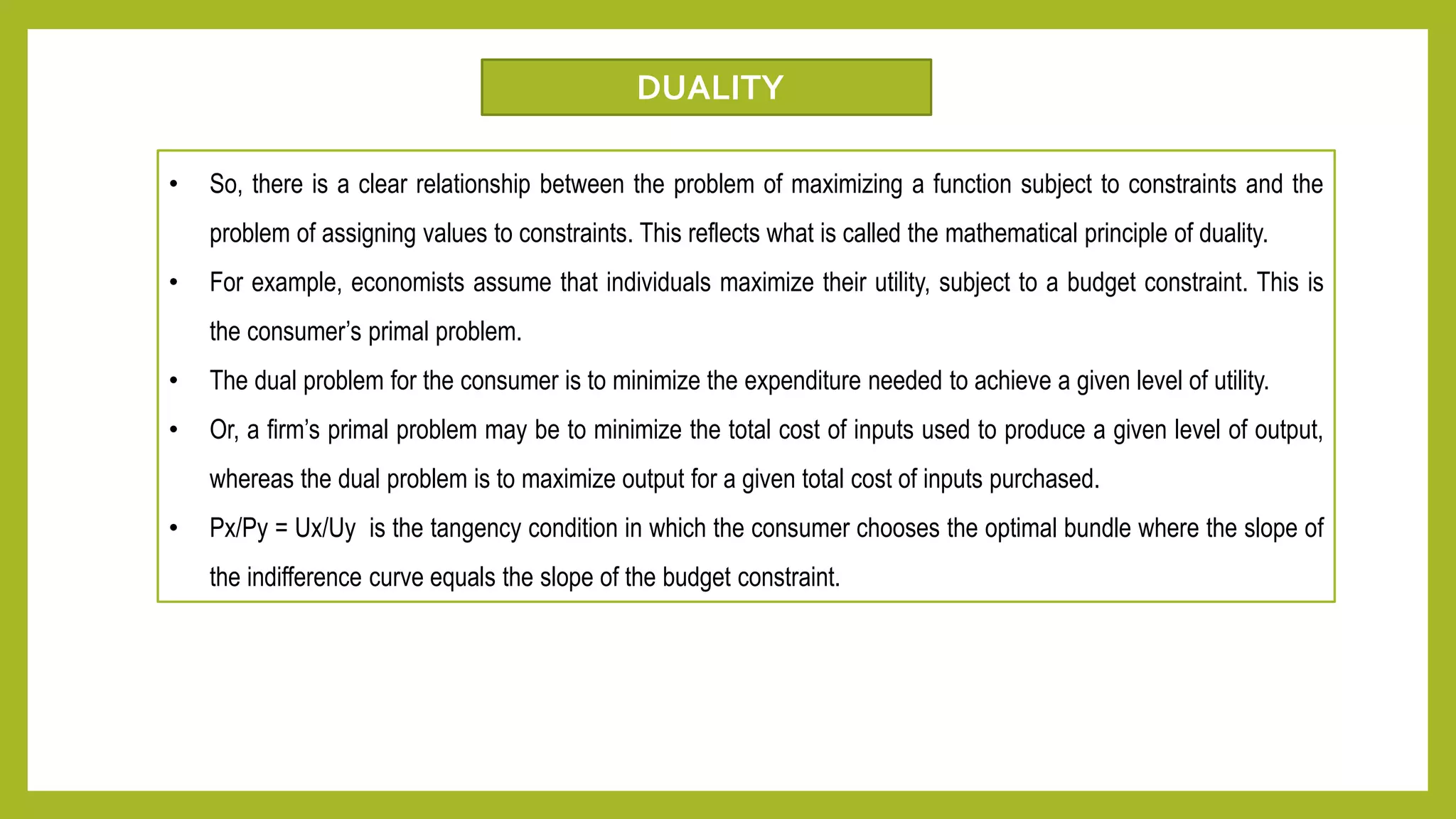
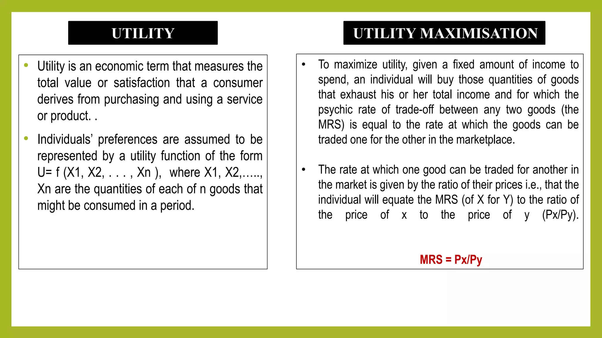
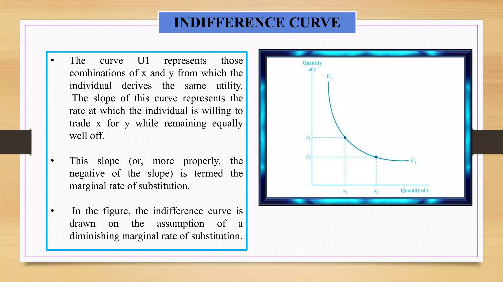
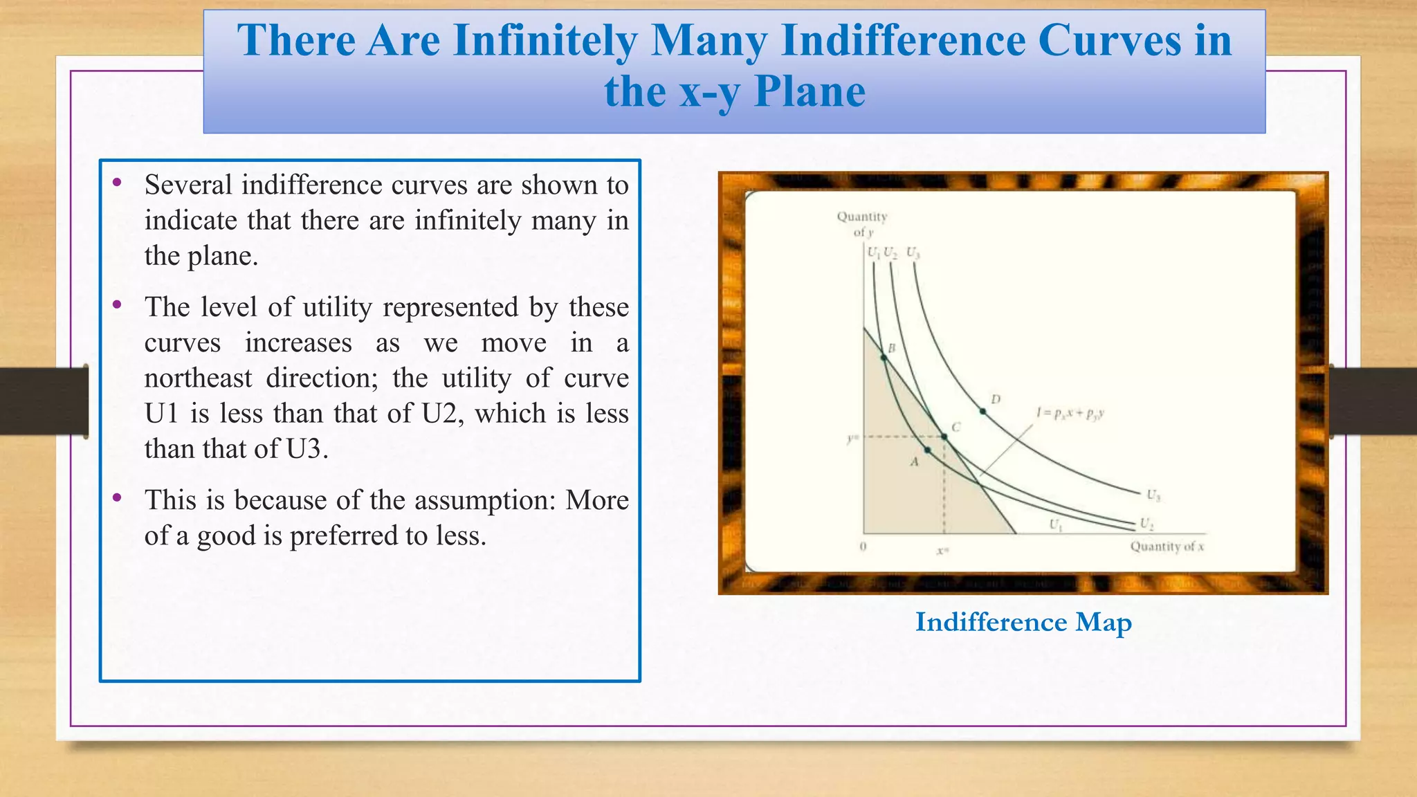
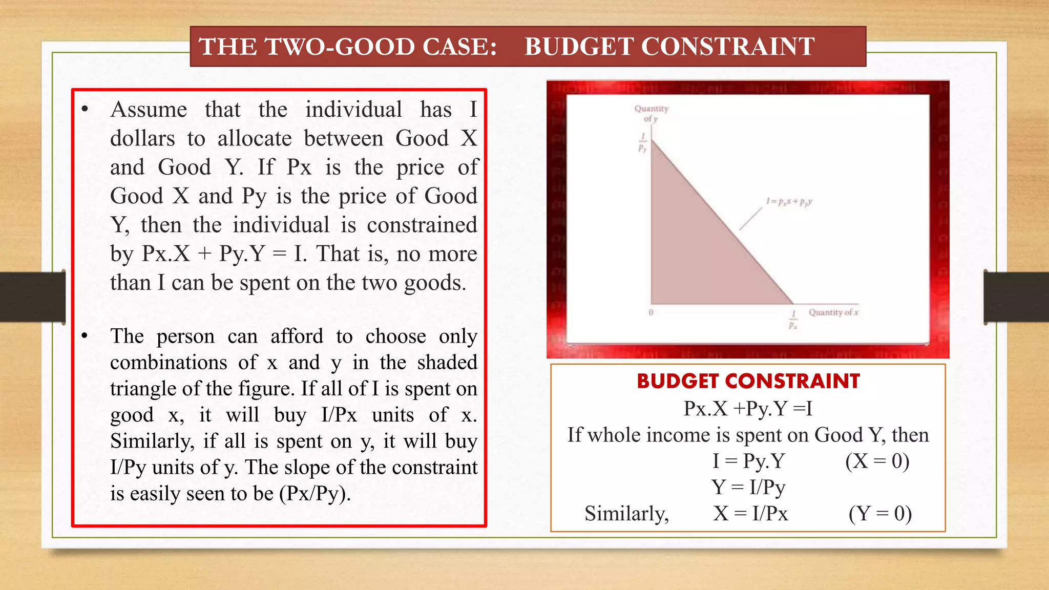
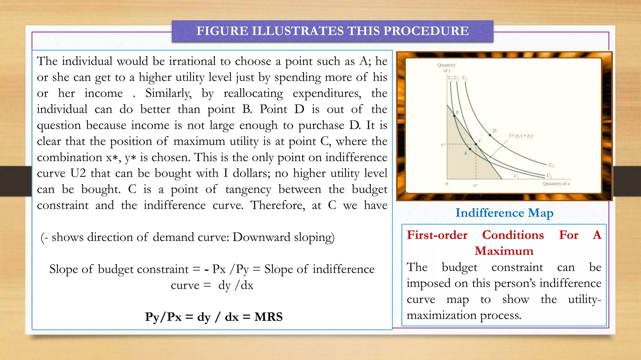
- Utility is a measure of satisfaction derived from consuming goods and services. Individuals seek to maximize their utility subject to a budget constraint. - Indifference curves represent combinations of goods that provide equal utility. The slope of the indifference curve is the marginal rate of substitution (MRS). - The budget constraint shows affordable combinations given prices and income. Utility is maximized at the point where the MRS equals the price ratio, where the indifference curve is tangent to the budget constraint. 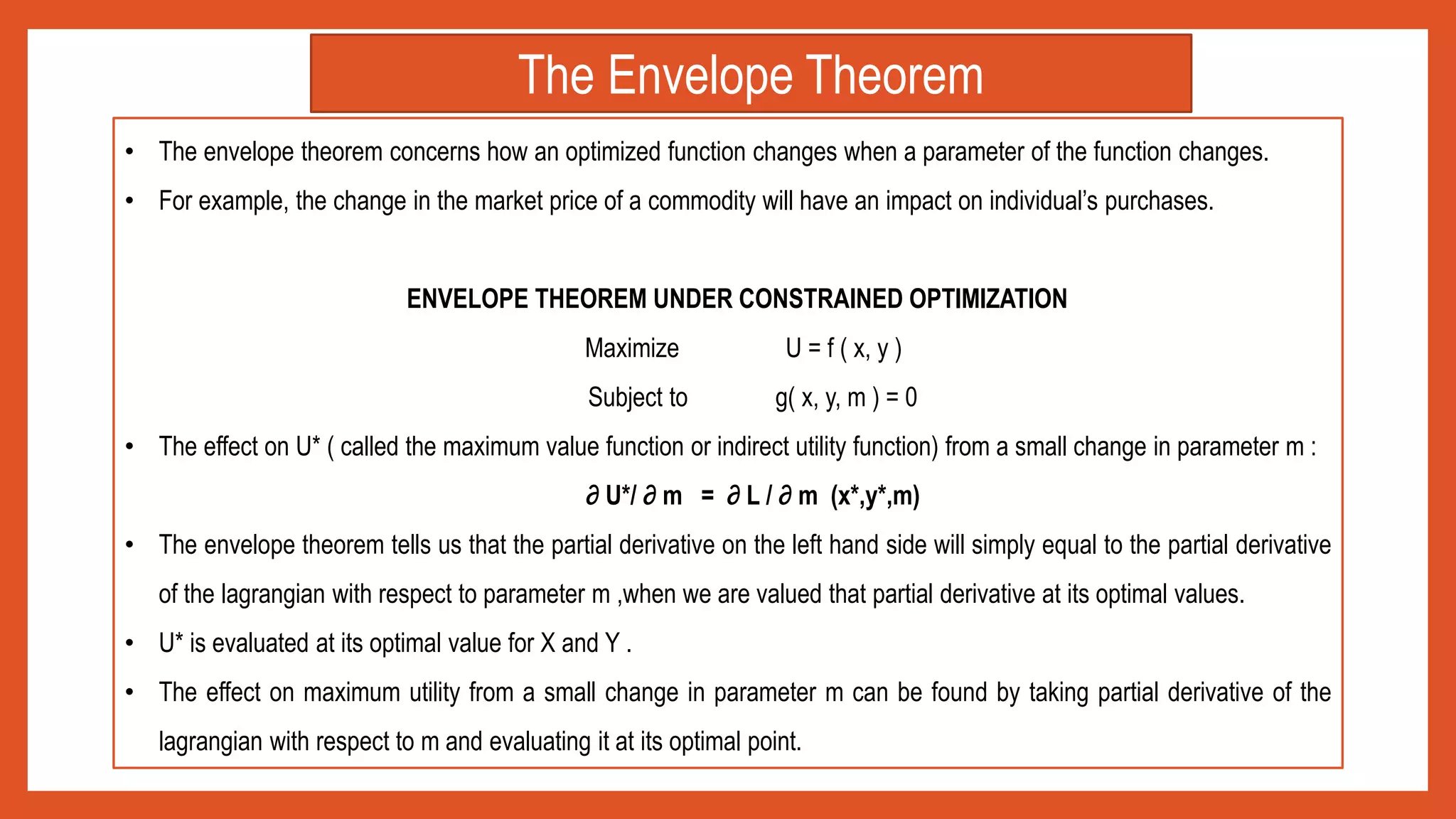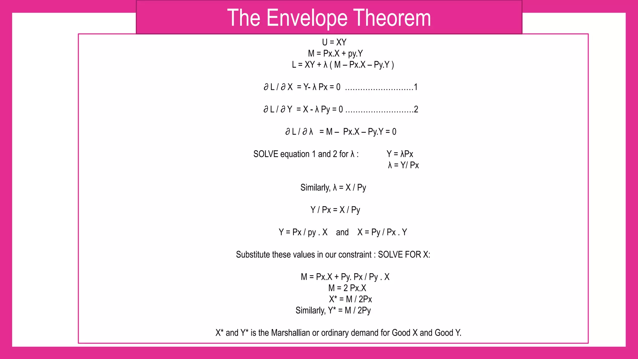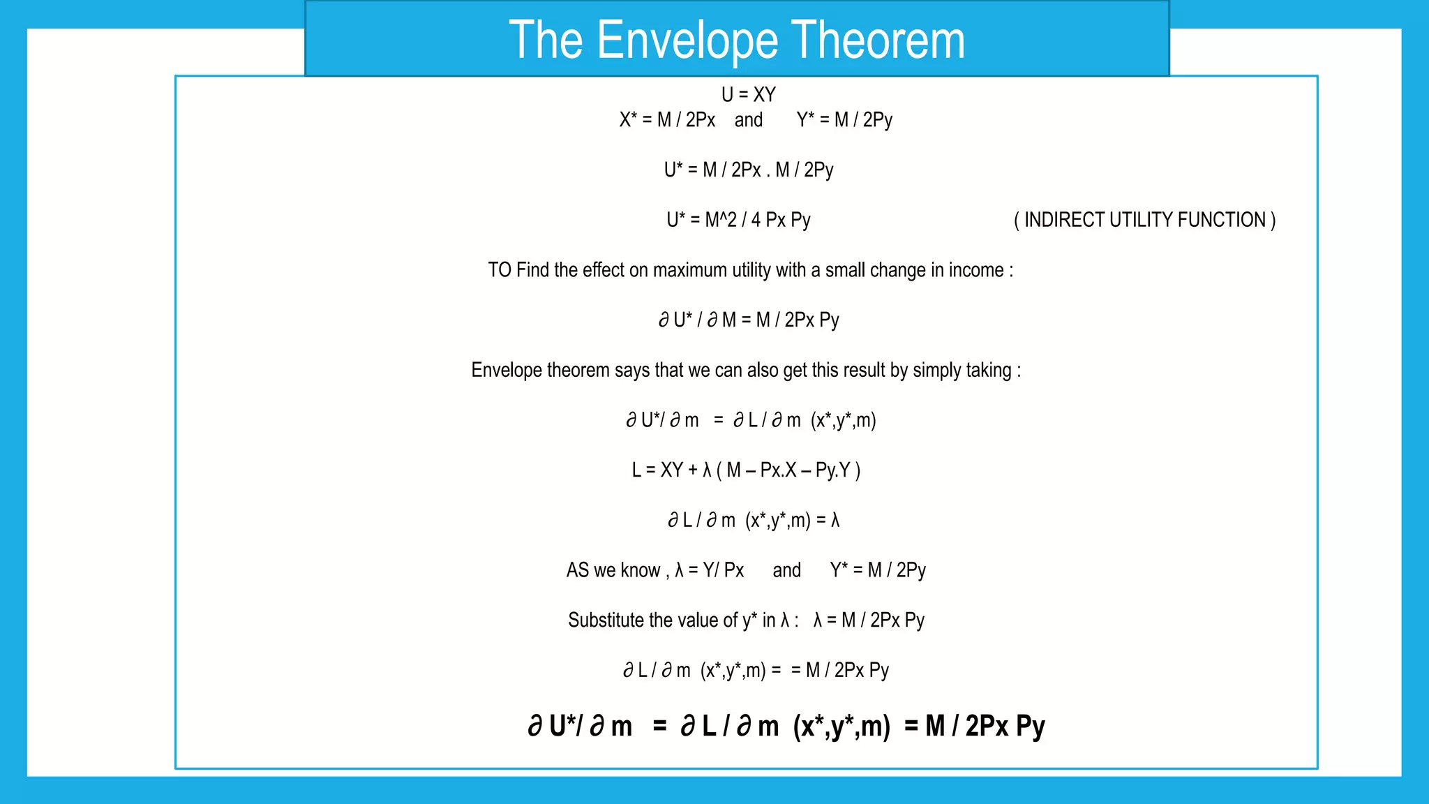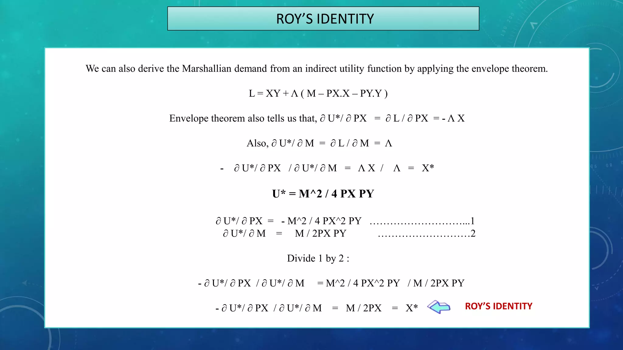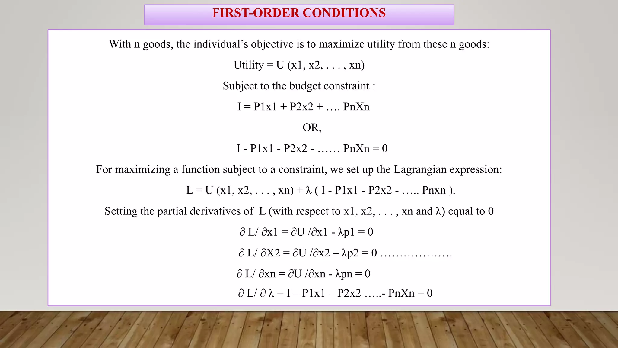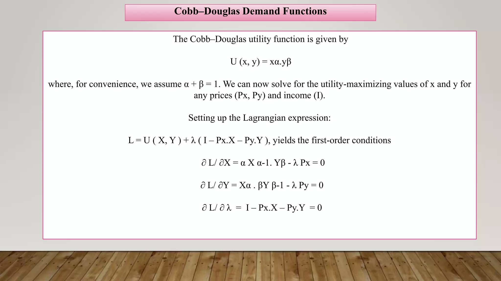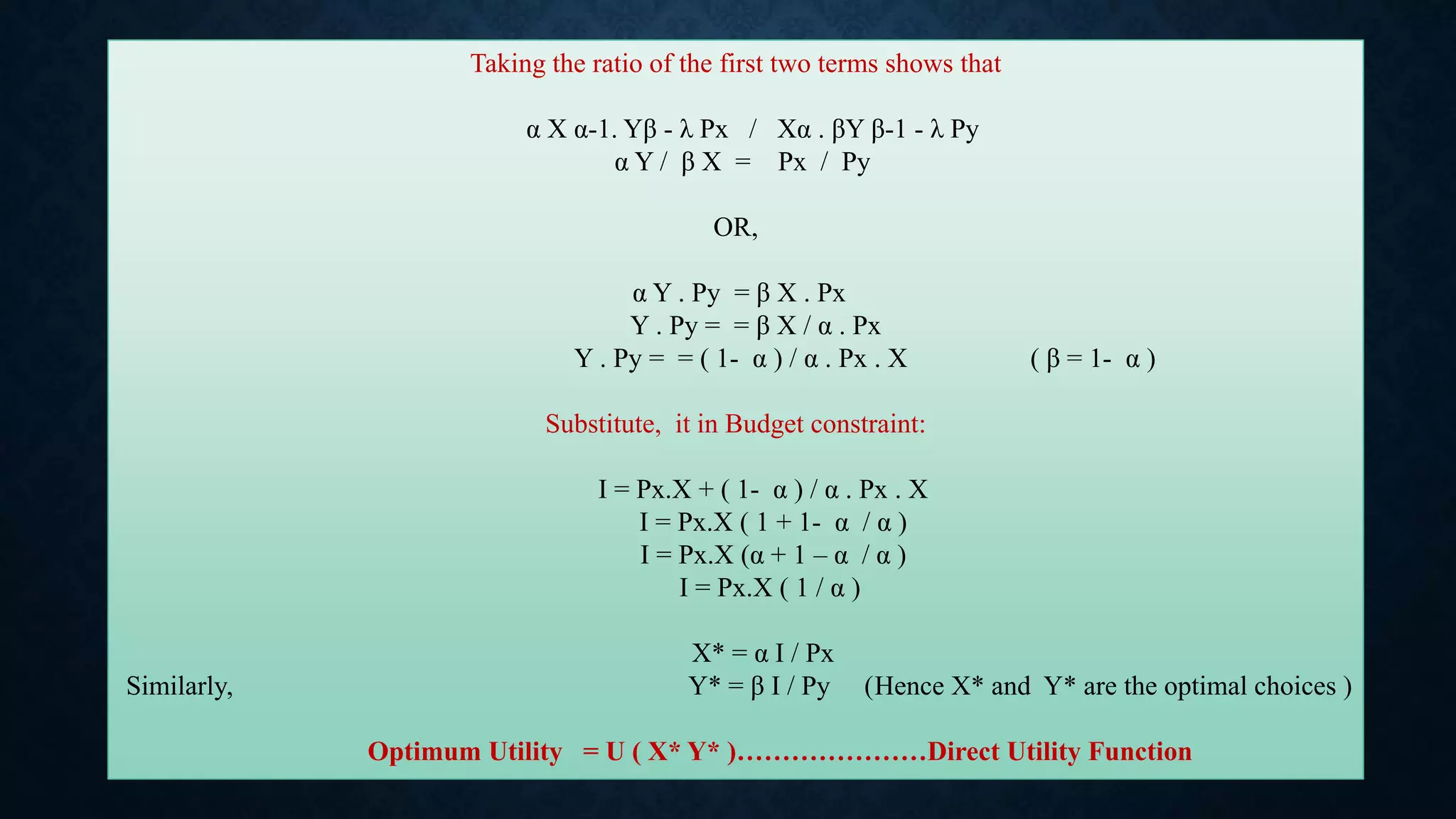- Using tools like Lagrangian optimization and the envelope theorem, the amounts demanded of each good can be derived as functions of prices and income.

3. • Utility is an economic term that measures the
total value or satisfaction that a consumer
derives from purchasing and using a service
or product. .
• Individuals’ preferences are assumed to be
represented by a utility function of the form
U= f (X1, X2, . . . , Xn ), where X1, X2,…..,
Xn are the quantities of each of n goods that
might be consumed in a period.
UTILITY
• To maximize utility, given a fixed amount of income to
spend, an individual will buy those quantities of goods
that exhaust his or her total income and for which the
psychic rate of trade-off between any two goods (the
MRS) is equal to the rate at which the goods can be
traded one for the other in the marketplace.
• The rate at which one good can be traded for another in
the market is given by the ratio of their prices i.e., that the
individual will equate the MRS (of X for Y) to the ratio of
the price of x to the price of y (Px/Py).
MRS = Px/Py
UTILITY MAXIMISATION

4. • The curve U1 represents those
combinations of x and y from which the
individual derives the same utility.
The slope of this curve represents the
rate at which the individual is willing to
trade x for y while remaining equally
well off.
• This slope (or, more properly, the
negative of the slope) is termed the
marginal rate of substitution.
• In the figure, the indifference curve is
drawn on the assumption of a
diminishing marginal rate of substitution.
INDIFFERENCE CURVE

5. • Assume that the individual has I
dollars to allocate between Good X
and Good Y. If Px is the price of
Good X and Py is the price of Good
Y, then the individual is constrained
by Px.X + Py.Y = I. That is, no more
than I can be spent on the two goods.
• The person can afford to choose only
combinations of x and y in the shaded
triangle of the figure. If all of I is spent on
good x, it will buy I/Px units of x.
Similarly, if all is spent on y, it will buy
I/Py units of y. The slope of the constraint
is easily seen to be (Px/Py).
THE TWO-GOOD CASE: BUDGET CONSTRAINT
BUDGET CONSTRAINT
Px.X +Py.Y =I
If whole income is spent on Good Y, then
I = Py.Y (X = 0)
Y = I/Py
Similarly, X = I/Px (Y = 0)

6. There Are Infinitely Many Indifference Curves in
the x-y Plane
• Several indifference curves are shown to
indicate that there are infinitely many in
the plane.
• The level of utility represented by these
curves increases as we move in a
northeast direction; the utility of curve
U1 is less than that of U2, which is less
than that of U3.
• This is because of the assumption: More
of a good is preferred to less.
Indifference Map

7. The individual would be irrational to choose a point such as A; he
or she can get to a higher utility level just by spending more of his
or her income . Similarly, by reallocating expenditures, the
individual can do better than point B. Point D is out of the
question because income is not large enough to purchase D. It is
clear that the position of maximum utility is at point C, where the
combination x∗, y∗ is chosen. This is the only point on indifference
curve U2 that can be bought with I dollars; no higher utility level
can be bought. C is a point of tangency between the budget
constraint and the indifference curve. Therefore, at C we have
(- shows direction of demand curve: Downward sloping)
Slope of budget constraint = - Px /Py = Slope of indifference
curve = dy /dx
Py/Px = dy / dx = MRS
FIGURE ILLUSTRATES THIS PROCEDURE
Indifference Map
First-order Conditions For A
Maximum
The budget constraint can be
imposed on this person’s indifference
curve map to show the utility-
maximization process.

8. With n goods, the individual’s objective is to maximize utility from these n goods:
Utility = U (x1, x2, . . . , xn)
Subject to the budget constraint :
I = P1x1 + P2x2 + …. PnXn
OR,
I - P1x1 - P2x2 - …… PnXn = 0
For maximizing a function subject to a constraint, we set up the Lagrangian expression:
L = U (x1, x2, . . . , xn) + λ ( I - P1x1 - P2x2 - ….. Pnxn ).
Setting the partial derivatives of L (with respect to x1, x2, . . . , xn and λ) equal to 0
∂ L/ ∂x1 = ∂U /∂x1 - λp1 = 0
∂ L/ ∂X2 = ∂U /∂x2 – λp2 = 0 ……………….
∂ L/ ∂xn = ∂U /∂xn - λpn = 0
∂ L/ ∂ λ = I – P1x1 – P2x2 …..- PnXn = 0
FIRST-ORDER CONDITIONS

9. The Cobb–Douglas utility function is given by
U (x, y) = xα.yβ
where, for convenience, we assume α + β = 1. We can now solve for the utility-maximizing values of x and y for
any prices (Px, Py) and income (I).
Setting up the Lagrangian expression:
L = U ( X, Y ) + λ ( I – Px.X – Py.Y ), yields the first-order conditions
∂ L/ ∂X = α X α-1. Yβ - λ Px = 0
∂ L/ ∂Y = Xα . βY β-1 - λ Py = 0
∂ L/ ∂ λ = I – Px.X – Py.Y = 0
Cobb–Douglas Demand Functions

10. Taking the ratio of the first two terms shows that
α X α-1. Yβ - λ Px / Xα . βY β-1 - λ Py
α Y / β X = Px / Py
OR,
α Y . Py = β X . Px
Y . Py = = β X / α . Px
Y . Py = = ( 1- α ) / α . Px . X ( β = 1- α )
Substitute, it in Budget constraint:
I = Px.X + ( 1- α ) / α . Px . X
I = Px.X ( 1 + 1- α / α )
I = Px.X (α + 1 – α / α )
I = Px.X ( 1 / α )
X* = α I / Px
Similarly, Y* = β I / Py (Hence X* and Y* are the optimal choices )
Optimum Utility = U ( X* Y* )…………………Direct Utility Function

11. In order to solve for the optimal values of x1, x2, . . . , xn.
These optimal values in general depends on the prices of all the goods and on the individual’s income. That is,
X1*= X1 (P1, P2, . . . , Pn, I ),
X2*= X2 (P1, P2, . . . , Pn, I ), ....
Xn*= Xn (P1, P2, . . . , Pn, I ),
These demand functions, shows the dependence of the quantity of each xi demanded on P1, P2, . . . , Pn and I.
Substitute the optimal values of the x’s to in the original utility function to yield maximum utility =
U [ X1* (P1, P2, . . . , Pn, I ), X2* (P1, P2, . . . , Pn, I ) ,… Xn* (P1, P2, . . . , Pn, I )] = V (P1, P2, . . . , Pn, I )
INDIRECT UTILITY FUNCTION

12. Now as we know that :
X* = α I / Px
Y* = β I / Py
Putting these values in the original utility function, we get:
U (x*,y*) = xα.yβ = (α I / Px) α . (β I / Py ) β
If, I = 8 , Px = 1 , Py = 4 , α +β = 1 (constant returns to scale)
U ( x*,y*) = x^0.5 . y^0.5 = [ 0.5 (8) / 1 ]^0.5 . [ 0.5 (8) / 4 ]^0.5 =

13. U = (X*,Y*)
Subject to constraint, Px + Py = I
Setting up the Lagrangian expression:
L = U ( X, Y ) + λ ( I – Px.X – Py.Y )
L = U ( X, Y ) + λ I – λPx.X – λPy
∂ L / ∂ Px = - λ x ------------ 1
∂ L / ∂ Py = - λ y ----------- 2
∂ L / ∂ I = λ ------------ 3
By Dividing equation 1 by 3, we get :
∂ L/ ∂ Px / ∂ L/ ∂ I = - λ X* / λ
- ∂ L/ ∂ Px / ∂ L/ ∂ I = X*
ROY’S IDENTITY
Roy’s Identity states that the individual consumers Marshallian demand function is equal to negative of the ratio of two partial
derivatives of the maximum value function.

14. DUALITY AND THE ENVELOPE THEOREM
• A consumer’s expenditure function and his/her indirect utility function exemplify
the minimum and maximum value functions for dual problems.
• An expenditure function specifies the minimum expenditure required to obtain a
fixed level of utility given the utility function and the prices of consumption goods.
• An indirect utility function specifies the maximum utility that can be obtained
given prices , income and utility function.

15. Let U(x,y) be a utility function where x and y are
consumption goods. The consumer has a budget B and
faces market prices Px and Py for goods X and Y ,
respectively. The problem will be considered the primal
problem:
Maximize U = U (x,y)
subject to Px.X + Py.Y = B [ PRIMAL]
THE PRIMAL PROBLEM
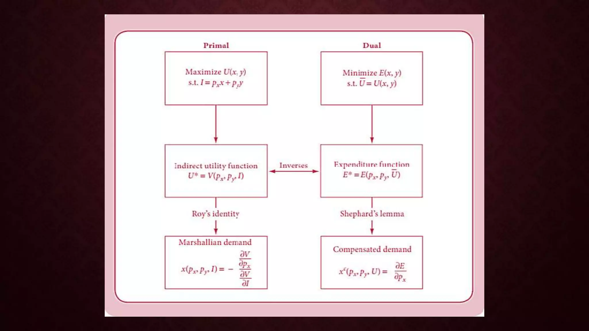
A related dual problem for the consumer with the objective of
minimising the expenditure on X and Y while maintaining a fixed
utility level u* derived from the primal problem:
Minimise E = Px.X + Py.Y
subject to U (x,y) = U* [ Dual ]
THE DUAL PROBLEM

16. • So, there is a clear relationship between the problem of maximizing a function subject to constraints and the
problem of assigning values to constraints. This reflects what is called the mathematical principle of duality.
• For example, economists assume that individuals maximize their utility, subject to a budget constraint. This is
the consumer’s primal problem.
• The dual problem for the consumer is to minimize the expenditure needed to achieve a given level of utility.
• Or, a firm’s primal problem may be to minimize the total cost of inputs used to produce a given level of output,
whereas the dual problem is to maximize output for a given total cost of inputs purchased.
• Px/Py = Ux/Uy is the tangency condition in which the consumer chooses the optimal bundle where the slope of
the indifference curve equals the slope of the budget constraint.
DUALITY

18. • The envelope theorem concerns how an optimized function changes when a parameter of the function changes.
• For example, the change in the market price of a commodity will have an impact on individual’s purchases.
ENVELOPE THEOREM UNDER CONSTRAINED OPTIMIZATION
Maximize U = f ( x, y )
Subject to g( x, y, m ) = 0
• The effect on U* ( called the maximum value function or indirect utility function) from a small change in parameter m :
∂ U*/ ∂ m = ∂ L / ∂ m (x*,y*,m)
• The envelope theorem tells us that the partial derivative on the left hand side will simply equal to the partial derivative
of the lagrangian with respect to parameter m ,when we are valued that partial derivative at its optimal values.
• U* is evaluated at its optimal value for X and Y .
• The effect on maximum utility from a small change in parameter m can be found by taking partial derivative of the
lagrangian with respect to m and evaluating it at its optimal point.
The Envelope Theorem

19. U = XY
M = Px.X + py.Y
L = XY + λ ( M – Px.X – Py.Y )
∂ L / ∂ X = Y- λ Px = 0 ………………………1
∂ L / ∂ Y = X - λ Py = 0 ………………………2
∂ L / ∂ λ = M – Px.X – Py.Y = 0
SOLVE equation 1 and 2 for λ : Y = λPx
λ = Y/ Px
Similarly, λ = X / Py
Y / Px = X / Py
Y = Px / py . X and X = Py / Px . Y
Substitute these values in our constraint : SOLVE FOR X:
M = Px.X + Py. Px / Py . X
M = 2 Px.X
X* = M / 2Px
Similarly, Y* = M / 2Py
X* and Y* is the Marshallian or ordinary demand for Good X and Good Y.
The Envelope Theorem

20. U = XY
X* = M / 2Px and Y* = M / 2Py
U* = M / 2Px . M / 2Py
U* = M^2 / 4 Px Py ( INDIRECT UTILITY FUNCTION )
TO Find the effect on maximum utility with a small change in income :
∂ U* / ∂ M = M / 2Px Py
Envelope theorem says that we can also get this result by simply taking :
∂ U*/ ∂ m = ∂ L / ∂ m (x*,y*,m)
L = XY + λ ( M – Px.X – Py.Y )
∂ L / ∂ m (x*,y*,m) = λ
AS we know , λ = Y/ Px and Y* = M / 2Py
Substitute the value of y* in λ : λ = M / 2Px Py
∂ L / ∂ m (x*,y*,m) = = M / 2Px Py
∂ U*/ ∂ m = ∂ L / ∂ m (x*,y*,m) = M / 2Px Py
The Envelope Theorem

21. We can also derive the Marshallian demand from an indirect utility function by applying the envelope theorem.
L = XY + Λ ( M – PX.X – PY.Y )
Envelope theorem also tells us that, ∂ U*/ ∂ PX = ∂ L / ∂ PX = - Λ X
Also, ∂ U*/ ∂ M = ∂ L / ∂ M = Λ
- ∂ U*/ ∂ PX / ∂ U*/ ∂ M = Λ X / Λ = X*
U* = M^2 / 4 PX PY
∂ U*/ ∂ PX = - M^2 / 4 PX^2 PY ………………………...1
∂ U*/ ∂ M = M / 2PX PY ………………………2
Divide 1 by 2 :
- ∂ U*/ ∂ PX / ∂ U*/ ∂ M = M^2 / 4 PX^2 PY / M / 2PX PY
- ∂ U*/ ∂ PX / ∂ U*/ ∂ M = M / 2PX = X*
ROY’S IDENTITY
ROY’S IDENTITY