The document summarizes key aspects of the gamma function. It begins by introducing the gamma function and defining it as the integral from 0 to infinity of t^x-1e^-t dt. It then establishes some key properties in 3 sentences or less: 1) The gamma function satisfies the functional equation gamma(x+1)=x*gamma(x) and can be interpreted as an extension of factorials to real and complex values. 2) Euler's beta function is introduced and shown to be related to the gamma function by the equation B(x,y)=gamma(x)*gamma(y)/gamma(x+y). 3) The gamma function is logarithmically convex, meaning the log

1. Chapter 2
The Gamma Function
In what follows, we introduce the classical Gamma function in Sect. 2.1. It is
essentially understood to be a generalized factorial. However, there are many further
applications, e.g., as part of probability distributions (see, e.g., Evans et al. 2000).
The main properties of the Gamma function are explained in this chapter (for
a more detailed discussion the reader is referred to, e.g., Artin (1964), Lebedev
(1973), M¨ ller (1998), Nielsen (1906), and Whittaker and Watson (1948) and
u
the references therein). We briefly consider Euler’s Beta function in Sect. 2.2 and
use it to recursively compute the volume of the .q 1/-dimensional unit sphere
Sq 1 Rq . As outstanding property of the Gamma function the Stirling formula is
verified in Sect. 2.3. It leads us to the so-called duplication formula (Lemma 2.3.3)
which will simplify a lot of calculations in later chapters. The extension of the
Gamma function to complex values is studied in Sect. 2.4. In doing so, we introduce
Pochhammer’s factorial and Euler’s constant . Moreover, we establish product
representations for the Gamma function as well as for trigonometric functions. In
Sect. 2.5 the incomplete Gamma and Beta functions are briefly presented in form of
some exercises and their relation to probability distributions is indicated.
2.1 Definition and Functional Equation
For real values x > 0, we consider the integrals
Z 1
e ttx 1
dt; (2.1.1)
0
and
Z 1
e ttx 1
dt: (2.1.2)
1
W. Freeden and M. Gutting, Special Functions of Mathematical (Geo-)Physics, 25
Applied and Numerical Harmonic Analysis, DOI 10.1007/978-3-0348-0563-6 2,
© Springer Basel 2013

2. 26 2 The Gamma Function
In order to show the convergence of (2.1.1) we observe that 0 < e t t x 1 Ä t x 1
holds true for all t 2 .0; 1. Therefore, for " > 0 sufficiently small, we have
Z Z ˇ
1
t x 1
1
x 1 t x ˇ1
ˇ D 1 "x
e t dt Ä t dt D : (2.1.3)
" " x ˇ" x x
Consequently, for all x > 0, the integral (2.1.1) is convergent. To assure the
convergence of (2.1.2) we observe that
1 1 nŠ
e ttx 1
D P1 tx 1
Ä tn
tx 1
D (2.1.4)
tk
kD0 kŠ nŠ
tn xC1
for all n 2 N and t 1. This shows us that
Z A Z A nCx ˇA
ˇ Â Ã
1 t ˇ D nŠ 1
e ttx 1
dt Ä nŠ dt D nŠ 1
1 1 tn xC1 x n ˇ1 x n An x
(2.1.5)
provided that A is sufficiently large and n is chosen such that n x C 1. Thus, the
integral (2.1.2) is convergent which we summarize in the following lemma.
Lemma 2.1.1. For all x > 0, the integral
Z 1
e ttx 1
dt (2.1.6)
0
is convergent.
Definition 2.1.2. The function x 7! .x/; x > 0, defined by
Z 1
.x/ D e ttx 1
dt (2.1.7)
0
is called the Gamma function (see Fig. 2.3 (right) for an illustration).
Obviously, we have the following properties:
(i) is positive for all x > 0,
R1
(ii) .1/ D 0 e t dt D 1.
We can use integration by parts to obtain for x > 0:
Z Z
1 ˇ1 1
.x C 1/ D e t t x dt D e t t x ˇ0 . e t /xt x 1
dt (2.1.8)
0 0
Z 1
Dx e ttx 1
dt D x .x/:
0

3. 2.1 Definition and Functional Equation 27
Lemma 2.1.3. The Gamma function satisfies the functional equation
.x C 1/ D x .x/; x > 0: (2.1.9)
Moreover, by iteration for x > 0 and n 2 N;
n
Y
.x C n/ D .x C n 1/ : : : .x C 1/x .x/ D .x C i 1/ .x/; (2.1.10)
i D1
ÂY Ã
n n
Y
.n C 1/ D i .1/ D i D nŠ: (2.1.11)
i D1 i D1
In other words, the Gamma function can be interpreted as an extension of factorials.
Lemma 2.1.4. The Gamma function is differentiable for all x > 0 and we have
Z 1
0 t
.x/ D e ln.t/t x 1
dt: (2.1.12)
0
Proof. For x > jhj > 0, we use the formula t y D eln.t /y , y > 0, t > 0:
Z 1 Z 1
t xCh 1
.x C h/ D e t dt D e t Cln.t /.xCh 1/ dt: (2.1.13)
0 0
By Taylor’s formula we find 0 < # < 1 such that
Z 1
.x C h/ .x/ D e t e ln.t / eln.t /.xCh/ eln.t /x dt (2.1.14)
0
Z 1
D e te ln.t /
h ln.t/t x C 1 h2 .ln.t//2 t xC#h dt
2
0
Z 1 Z 1
t x 1 1 2
Dh e ln.t/t dt C 2h e t .ln.t//2 t xC#h 1
dt:
0 0
This gives us the differentiability of if the second integral is bounded. Consider
the following estimate (we employ that .ln.t//2 Ä t 2 for t 1 and that e t Ä 1 for
t 2 Œ0; 1/
Z 1 Z 1 Z 1
e t .ln.t//2 t xC#h 1
dt D e t .ln.t//2 t xC#h 1
dt C e t .ln.t//2 t xC#h 1
dt
0 0 1
Z 1 Z 1
Ä .ln.t//2 t xC#h 1
dt C e t t 2 t xC#h 1
dt
0 1
2
Ä .2 C x C #h/ C < 1: (2.1.15)
.x C #h/3
This provides us with the desired result. t
u

4. 28 2 The Gamma Function
An analogous proof can be given to show that is infinitely often differentiable for
all x > 0 and Z 1
.k/
.x/ D e t .ln.t//k t x 1
dt; k 2 N: (2.1.16)
0
Lemma 2.1.5 (Gauß’ Expression of the Second Logarithmic Derivative). For
x > 0,
0 2
.x/ < .x/ 00 .x/: (2.1.17)
Equivalently, we have
 Ã2 00  0 Ã2
d .x/ .x/
ln. .x// D > 0; (2.1.18)
dx .x/ .x/
i.e., x 7! ln. .x//, x > 0, is a convex function or is logarithmic convex.
Proof. We start with
ÂZ 1 Ã2
0 2 t
.x/ D e ln.t/t x 1
dt
0
ÂZ 1 Ã2
t x 1 t x 1
D e 2 t 2 ln.t/e 2 t 2 dt : (2.1.19)
0
The Cauchy–Schwarz inequality yields (note that equality cannot occur since the
two functions are linearly independent):
Z 1 Á2 Z 1 Á2
0 2 t x 1 t x 1
.x/ < e 2 t 2 dt e 2 t 2 ln.t/ dt
0 0
Z 1 Z 1
t x 1
D e t dt e ttx 1
.ln.t//2 dt D .x/ 00
.x/: (2.1.20)
0 0
Moreover, we find with the help of (2.1.20) that
d2 d 0
.x/ 00
.x/ .x/ . 0
.x//2
ln. .x// D D > 0; (2.1.21)
dx 2 dx .x/ . .x//2
which yields (2.1.18). t
u
Note that ln. . // is convex, i.e., for t 2 Œ0; 1
ln . .tx C .1 t/y// Ä t ln. .x// C .1 t/ ln. .y//
t 1 t
D ln .x/ C ln .y/
t 1 t
D ln .x/ .y/ (2.1.22)
t 1 t
which is equivalent to .tx C .1 t/y/ Ä .x/ .y/ with x; y > 0.

5. 2.2 Euler’s Beta Function 29
Fig. 2.1 The illustration of the coordinate transformation relating the Beta and the Gamma
functions
2.2 Euler’s Beta Function
Next, we notice that for x; y > 0; the integral
Z 1
tx 1
.1 t/y 1
dt (2.2.1)
0
is convergent.
Definition 2.2.1. The function .x; y/ 7! B.x; y/, x; y > 0, defined by
Z 1
B.x; y/ D tx 1
.1 t/y 1
dt (2.2.2)
0
is called the Euler Beta function.
For x; y > 0, we see that
Z 1 Z 1 Z 1 Z 1
.x/ .y/ D e ttx 1
dt e s sy 1
ds D e .t Cs/ x 1 y 1
t s dt ds:
0 0 0 0
(2.2.3)
Note that the transition from one-dimensional to two-dimensional integrals is
permitted by Fubini’s theorem. We make a coordinate transformation (see Fig. 2.1)
as follows:
t D u.1 v/; 0 Ä u < 1; (2.2.4)
s D uv; 0 Ä v Ä 1: (2.2.5)
It is not difficult to verify that the functional determinant of the coordinate
transformation is given by
ˇ ˇ
@.t; s/ ˇ1 v uˇ
Dˇˇ ˇ D u.1 v/ C uv D u 0: (2.2.6)
@.u; v/ v uˇ

6. 30 2 The Gamma Function
Thus, we find
Z 1 Z 1 Z 1 Z 1
.t Cs/ x 1 y 1
e t s dt ds D e u .u.1 v//x 1 .uv/y 1 u du dv
0 0 0 0
Z 1 Z 1
D e u uxCy 2 .1 v/x 1 vy 1 u du dv
0 0
Z 1 Z 1
D e u uxCy 1
du vy 1 .1 v/x 1
dv:
0 0
(2.2.7)
This leads us to the following theorem:
Theorem 2.2.2. For x; y > 0,
.x/ .y/
B.x; y/ D : (2.2.8)
.x C y/
In particular,
 à Z 1 Z 1
1 1 1 1 1
B ; D t 2 .1 t/ 2 dt D 2 .1 u2 / 2 du (2.2.9)
2 2 0 0
D 2 arcsin.1/ D 2 D :
2
Therefore, we have
2 1
2
D : (2.2.10)
.1/
This shows that
 à Z 1
1 p 1
D D e tt 2 dt: (2.2.11)
2 0
Other types of integrals can be derived from
Z 1 Z 1 Â Ã
t˛ 1
uDt ˛ 1
1 1 1
e dt D e u u ˛ du D ; ˛ > 0: (2.2.12)
0 ˛ 0 ˛ ˛
Lemma 2.2.3. For ˛ > 0,
Z 1 Â Ã
t˛ ˛C1
e dt D : (2.2.13)
0 ˛

7. 2.2 Euler’s Beta Function 31
In particular, Lemma 2.2.3 yields for ˛ D 2
Z 1 Â Ã Â Ã p
t2 3 1 1
e dt D D D : (2.2.14)
0 2 2 2 2
Moreover, we have
Z 1
t˛ 1 xÁ
tx 1
e dt D ; x; ˛ > 0; (2.2.15)
0 ˛ ˛
and
Z 1
˛t 2 1 x xÁ
tx 1
e dt D ˛ 2 ; x; ˛ > 0: (2.2.16)
0 2 2
Within the notational framework of polar coordinates (see (6.1.17) and (6.1.18) for
details) we are now prepared to give the well-known calculation of the area kSq 1 k
of the unit sphere Sq 1 in Rq : By definition, we set kS0 k D 2. Clearly, S1 is the unit
circle in R2 , i.e., S1 D fx 2 R2 W jxj D 1g. Hence, its area is equal to
kS1 k D 2 : (2.2.17)
Furthermore, S2 D fx 2 R3 W jxj D 1g is the unit sphere in R3 . Thus, its area is
known to be equal to
kS2 k D 4 : (2.2.18)
We are interested in deriving the area of the sphere Sq 1
in Rq .q > 3/:
Z
q 1
kS kD dS.q 1/ . .q/ /: (2.2.19)
Sq 1
In terms of spherical coordinates (6.1.17) and (6.1.18) in Rq the surface element
dS.q 1/ . / of the sphere Sq 1 in Rq admits the representation
p Á
dS.q 1/ .q/ D dS.q 2/ 1 t2 .q 1/ dt (2.2.20)
p Á
C . 1/q 1 t dV.q 1/ 1 t2 .q 1/ :
Now, we notice that
p Á q 3
dV.q 1/ 1 t2 .q 1/ D t.1 t 2/ 2 dt dS.q 2/ .q 1/ (2.2.21)
q 3
D . 1/q 1 t.1 t 2/ 2 dS.q 2/ .q 1/ dt:

8. 32 2 The Gamma Function
In addition, it is not difficult to see that
p Á q 1
dS.q 2/ 1 t 2 .q 1/ D .1 t 2/ 2 dS.q 2/ .q 1/ : (2.2.22)
Combining our results we are led to the identity
p Á
dS.q 1/ t "q C 1 t2 .q 1/ (2.2.23)
q 3
D .1 t 2/ 2 1 t 2 C t 2 dS.q 2/ .q 1/ dt;
p
where we have used the decomposition .q/ D t "q 1 t 2 .q 1/ . Note that "1 ; : : : ; "q
is the canonical orthonormal system in Rq . In brief, we obtain
q 3
dS.q 1/ .q/ D .1 t 2/ 2 dS.q 2/ .q 1/ dt; (2.2.24)
such that
Z 1 Z
q 3
kSq 1
kD .1 t 2/ 2 dS.q 2/ . .q 1/ / dt (2.2.25)
1 Sq 2
Z 1 q 3
D kSq 2
k .1 t 2/ 2 dt:
1
For the computation of the remaining integral it is helpful to use some facts known
from the Gamma function as well as Euler’s Beta function. More explicitly,
Z 1 Z 1 Z 1
2
q 3
2
q 3 t 2 Dv 1 q 3
.1 t / 2 dt D 2 .1 t / 2 dt D v 2 .1 v/ 2 dv (2.2.26)
1 0 0
Á p Á
 à 1 q 1 q 1
1 q 1 2 2 2
DB ; D q D q :
2 2 2 2
By recursion we get the following lemma from (2.2.26):
Lemma 2.2.4. For q 2,
q
2
q 1
kS kD2 q : (2.2.27)
2
q 1
The area of the sphere SR .y/ with center y 2 Rq and radius R > 0 is given by
q
2
q 1
kSR .y/k D kSq 1 k Rq 1
D2 q Rq 1 : (2.2.28)
2

9. 2.3 Stirling’s Formula 33
x q
Furthermore, using .q/ D jxj
, the volume of the ball BR .y/ with center y 2 Rq and
radius R > 0 is given by
Z Z R ÂZ Ã
q
kBR .y/k D dV.q/ .x/ D dS.q 1/ . .q/ / dr (2.2.29)
q q 1
BR .y/ rD0 Sr .y/
q Z R q
2 2
q 1
D2 q r dr D q Rq :
2 0 2
C1
2.3 Stirling’s Formula
Next, we are interested in the behavior of the Gamma function for large positive
values x. This provides us with the so-called Stirling’s formula, a result which we
apply to verify the helpful duplication formula and to extend the Gamma function
in Sect. 2.4.
Theorem 2.3.1 (Stirling’s Formula). For x > 0,
ˇ ˇ r
ˇ .x/ ˇ 2
ˇp 1ˇ Ä : (2.3.1)
ˇ 2 x x 1=2 e x ˇ x
Proof. Regard x as fixed and substitute
dt
t D x.1 C s/; 1 Ä s < 1; Dx (2.3.2)
ds
in the defining integral of the Gamma function. We obtain
Z 1 Z 1
.x/ D e ttx 1
dt D e x xs x 1
x .1 C s/x 1 x ds (2.3.3)
0 1
Z 1
x x
Dx e .1 C s/x 1
e xs
ds D x x e x
I.x/:
1
Our aim is to verify that I.x/ satisfies
ˇ r ˇ
ˇ 2 ˇ 2
ˇ ˇ
ˇI.x/ ˇÄ : (2.3.4)
ˇ x ˇ x
such that
ˇ r ˇ ˇ ˇ r
ˇ .x/ 2 ˇ 2 ˇ .x/ ˇ 2
ˇ ˇ
ˇ x x ˇÄ ; i:e:; ˇ
ˇ xx p 1ˇ Ä
ˇ : (2.3.5)
ˇx e x ˇ x 1=2 e x 2 x

10. 34 2 The Gamma Function
5
4
3
2
1
0
−1
−2
−3
−1 0 1 2 3 4 5 6
Fig. 2.2 The functions s 7! u2 .s/ D s ln.1 C s/ (blue) and u.s/ defined by (2.3.7) (red)
For that purpose we write
xu2 .s/
.1 C s/x e xs
D exp . x.s ln.1 C s/// D e ; (2.3.6)
where (cf. Fig. 2.2)
( 1
js ln.1 C s/j 2 ; s 2 Œ0; 1/;
u.s/ D 1 (2.3.7)
js ln.1 C s/j 2 ; s 2 . 1; 0/:
We set up the Taylor expansion of u2 for s 2 . 1; 1/ at 0:
du2 d2 u2 s2
u2 .s/ D u2 .0/ C.0/s C .#s/ (2.3.8)
ds ds 2 2
 Ã
1 1 s2
D0C 1 sC ;
1C0 .1 C s#/2 2
where # 2 .0; 1/. Therefore,
s2 1
u2 .s/ D (2.3.9)
2 .1 C s#/2
with 0 < # < 1. We interpret # as a uniquely defined function of s, i.e., # W s 7!
#.s/; such that

11. 2.3 Stirling’s Formula 35
u.s/ 1 1
D p (2.3.10)
s 2 .1 C s#.s//
is a positive continuous function for s 2 . 1; 1/ with the property
ˇ ˇ ˇ Â Ãˇ ˇ ˇ
ˇ u.s/ 1 ˇ ˇ 1 1 ˇ 1 ˇ ˇ
ˇ ˇ D ˇp
p ˇ ˇ ˇ D p ˇ s#.s/ ˇ
1 ˇ
ˇ s 2 2 1 C s#.s/ 2 ˇ 1 C s#.s/ ˇ
ˇ ˇ
ˇ s#.s/u.s/ ˇ
Dˇˇ
ˇ D j#.s/j ju.s/j Ä ju.s/j:
ˇ (2.3.11)
s
From u2 .s/ D s ln.1 C s/ follows that
s
2u du D ds: (2.3.12)
1Cs
Obviously, s W u 7! s.u/; u 2 R, is of class C.1/ .R/ and thus,
Z 1 Z C1
xu2 u
I.x/ D .1 C s/x 1 e xs
ds D 2 e du: (2.3.13)
1 1 s.u/
We are able to deduce that
ˇ ˇ ˇ ˇ
ˇ p Z 1 xu2 ˇ ˇ Z 1
u p Z C1 xu2 ˇ
ˇI.x/ 2 2 e duˇ D ˇ2 du
e xu2
2 e duˇ
ˇ ˇ ˇ s.u/ ˇ
0 1 1
ˇ Z Â Ã ˇ
ˇ 1
u 1 ˇ
D ˇ2 duˇ
2
ˇ e xu p ˇ
1 s.u/ 2
Z 1 ˇ ˇ
2 ˇ u 1 ˇ
Ä2 e xu ˇ ˇ
ˇ s.u/ p2 ˇ du
1
Z 1 Z 1
xu2 2
Ä2 e juj du D 4 e xu u du: (2.3.14)
1 0
Note that we can use the integral (2.2.16) with ˛ D x and x D 1;
Z 1 Z 1 p
xu2 xu2
u1 1 e du D e du D 1
2 x 1=2 1
2 D p ; (2.3.15)
0 0 2 x
as well as with ˛ D x and x D 2 in (2.2.16)
Z 1 Z 1
2 1 xu2 xu2 1 1 1
u e du D e u du D 2 x .1/ D : (2.3.16)
0 0 2x

12. 36 2 The Gamma Function
This yields:
ˇ r ˇ ˇ r ˇ
ˇ p 1 ˇ ˇ 2 ˇ 1 2
ˇI.x/ 2 2 ˇ D ˇI.x/
ˇ
ˇ
ˇÄ4 D : (2.3.17)
ˇ 2 xˇ ˇ x ˇ 2x x
This leads to the desired result. t
u
Remark 2.3.2. Stirling’s formula can be rewritten in the form
.x/
lim p D 1: (2.3.18)
x!1 2 xx 1=2 e x
An immediate application is the limit relation
.x C a/
lim D 1; a > 0: (2.3.19)
x!1 x a .x/
This can be seen from Stirling’s formula by
.x C a/
lim p 1
D1 (2.3.20)
x!1 2 .x C a/xCa 2 e x a
due to the relation
1 1 1
.x C a/xCa 2 D x xCa 2 .1 C x /xCa
a 2 (2.3.21)
and the limits
a
.1 C x /x 1
lim D 1; lim .1 C x /a
a 2 D 1: (2.3.22)
x!1 ea x!1
Next, we prove the so-called Legendre relation or duplication formula.
Lemma 2.3.3 (Duplication Formula). For x > 0 we have
 Ã
x 1 xÁ xC1 p
2 D .x/: (2.3.23)
2 2
Proof. We consider the function x 7! ˚.x/; x > 0; defined by
2x 1
. x / . xC1 /
2 2
˚.x/ D (2.3.24)
.x/
for x > 0. Setting x C 1 instead of x we find the following functional equation for
the numerator
 à Á  Ã
xC1 x xÁ xC1
2x C 1 D 2x 1 x ; (2.3.25)
2 2 2 2

13. 2.3 Stirling’s Formula 37
such that the numerator satisfies the same functional equation as the denominator.
This means ˚.x C 1/ D ˚.x/; x > 0. By repetition we get for all n 2 N and x
fixed ˚.x C n/ D ˚.x/. We let n tend to 1. For the numerator of ˚.x C n/ we
then find by use of the result in Remark 2.3.2, i.e., by using (2.3.19) twice, that
2xCn 1
. xCn / . xCnC1 /
2 2
lim x xC1 2
D 1: (2.3.26)
n!1 n
2xCn 1
2
2
.n/
2
2 .n/
2
For the denominator we consider
.x C n/
lim x xC1 2
n!1 xCn 1 n
2 2
2
.n/
2
2 .n/
2
.x C n/
D lim 2
n!1 1
n xC 2 ..n/ /
2xCn 1
2 . n /n 1 e
2
n2
n n 1
.2/
2
e n2
2
! 1
.x C n/ .n/
2
D lim
n!1
2xCn n nCx
1
2
e n . n /n 1 e n 2
2
2
2
! 1
.x C n/ .n/
2
D lim p p
n!1 2 nnCx
1
2 e n . n /n 1 e n 2
2
1
Dp ; (2.3.27)
since Stirling’s formula yields that
.n/
2
lim D 1; (2.3.28)
n!1 p n 1 n
2 .n/2
2
2e 2
i.e.,
2
.n/
2
lim D 1; (2.3.29)
n!1 2 . n /n 1 e n
2
and by the same arguments as in Remark 2.3.2 (set a in (2.3.20) to x and x
in (2.3.20) to n) we find that
.x C n/
lim p 1
D 1: (2.3.30)
n!1 2 nnCx 2 e n
Therefore, we get for every x > 0 and all n 2 N;
p
˚.x/ D ˚.x C n/ D lim ˚.x C n/ D : (2.3.31)
n!1

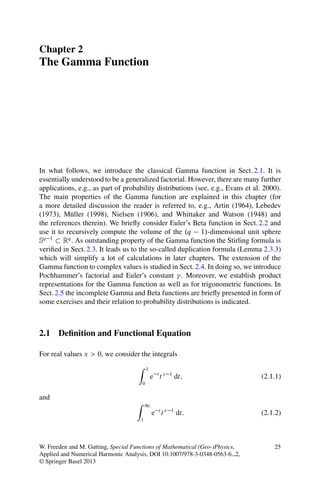
14. 38 2 The Gamma Function
A periodic function with this property must be constant. This proves the lemma. u
t
A generalization of the Legendre relation (“duplication formula”) is the Gauß
multiplication formula that can be verified by analogous arguments.
Lemma 2.3.4. For x > 0 and n 2,
 à  Ã
xÁ xC1 xCn 1 n 1 p
::: nx D .2 / 2 n .x/ : (2.3.32)
n n n
2.4 Pochhammer’s Factorial
Thus far, the Gamma function is defined for positive values, i.e., x 2 R>0 . We are
interested in an extension of to the real line R (or even to the complex plane C)
if possible.
Definition 2.4.1. The so-called Pochhammer factorial .x/n with x 2 R and n 2 N
is defined by
n
Y
.x/n D x.x C 1/ : : : .x C n 1/ D .x C i 1/: (2.4.1)
i D1
For x > 0, it is clear that
.x C n/
.x/n D (2.4.2)
.x/
or
.x/n 1
D : (2.4.3)
.x C n/ .x/
The left-hand side is defined for x > n and gives the same value for all n 2 N
1
with n > x. We may use this relation to define .x/ for all x 2 R, and we see that
this function vanishes for x D 0; 1; 2; : : : (see Fig. 2.3 (left)). We know that the
Gamma integral is absolutely convergent for x 2 C with Re.x/ > 0 and represents
a holomorphic function for all x 2 C with Re.x/ > 0. Moreover, the Pochhammer
factorial .x/n can be defined for all complex x. Because of (2.4.3) with n chosen
1
sufficiently large, we have a definition of .x/ for all x 2 C. This is summarized in
the following lemma.
Lemma 2.4.2. The -function is a meromorphic function that has simple poles in
1
0; 1; 2; : : : (see Fig. 2.3 (right)). The reciprocal x 7! .x/ is an entire analytic
function (see Fig. 2.3 (left) for an illustration).

15. 2.4 Pochhammer’s Factorial 39
5 10
4 8
6
3
4
2 2
1 0
0 −2
−4
−1
−6
−2 −8
−3 −10
−4 −3 −2 −1 0 1 2 3 4 5 −5 −4 −3 −2 −1 0 1 2 3 4 5
Fig. 2.3 The reciprocal of the Gamma function (left) and the Gamma function (right) on the real
line R
Lemma 2.4.3. For x 2 C,
n 1
Y
1 x x
D lim n x 1C k : (2.4.4)
.x/ n!1
kD1
Proof. Because of (2.4.3) the identity
.x/n .n/ 1
D (2.4.5)
.n/ .x C n/ .x/
is valid for all x 2 C with Re.x/ > n. Furthermore it is easy to see that
xÁ
n 1
Y
.x/n .x C 1/.x C 2/ : : : .x C n 1/
Dx Dx 1C : (2.4.6)
.n/ 1 2 : : : .n 1/ k
kD1
x
Combining the two and multiplying with n we find that
xÁ
n 1
Y
.x C n/ x
Dn x 1C : (2.4.7)
nx .n/ .x/ k
kD1
Now, we use (2.3.19) with x D n and a D x, i.e.,
.x C n/
lim D 1; x > 0; (2.4.8)
n!1 .n/nx
on the left-hand side and obtain for x > 0;
xÁ
n 1
Y
1 .x C n/ 1 x
D lim D lim n x 1C ; (2.4.9)
.x/ n!1 nx .n/ .x/ n!1 k
kD1

16. 40 2 The Gamma Function
which proves Lemma 2.4.3 for x > 0. To determine if this limit is also defined
for x Ä 0 we consider once again s ln.1 C s/ (cf. Fig. 2.2) with 1 < s < 1
from (2.3.9) in the proof of Theorem 2.3.1:
s2 1
0Äs ln.1 C s/ D ; # D #.s/ 2 .0; 1/: (2.4.10)
2 .1 C #s/2
1
Therefore, we can put s D k and estimate the right-hand side with its maximum,
i.e., with # D 0:
1 1 1
0Ä k
ln 1 C k
Ä 2k 2
: (2.4.11)
1P
n
1
This immediately proves that lim ln 1 C exists and is positive.
n!1 kD1 k k
Moreover,
n
X n
X
1 1 1
lim k ln 1 C k D lim k ln.k C 1/ C ln.k/
n!1 n!1
kD1 kD1
ÂX
n Ã
1
D lim k ln.n C 1/ D ; (2.4.12)
n!1
kD1
where denotes Euler’s constant
Âm 1
X Ã
1
D lim ln m 0:577215665 : : : : (2.4.13)
m!1 k
kD1
Assume now that x 2 R. If k 2jxj, then
x x x2
0Ä k ln 1 C k < k2
(2.4.14)
and
xÁ Y xÁ x xÁ
n 1
Y n 1 n 1
Y x n 1
Y
x x
1C D 1C ek e k D ej 1C e k: (2.4.15)
k k j D1
k
kD1 kD1 kD1
For k k0 D b2jxjc, we obtain by multiplying (2.4.14) with 1 and applying the
exponential function to it:
x x2
x
1 1C k
e k >e k2 ; (2.4.16)

17. 2.4 Pochhammer’s Factorial 41
which shows that
n 1
Y 1
Y
x x
x x
lim 1C k e k D 1C k e k (2.4.17)
n!1
kD1 kD1
exists for all x. Furthermore,
n 1
Y x
 X Ã
n 1 Â Xn 1 Ã
1 1
ej D exp x j D exp x j x ln.n/ C x ln.n/
j D1 j D1 j D1
 Xn 1 Ã
x 1
D n exp x j
x ln.n/ ; (2.4.18)
j D1
where
 Xn 1 Ã
lim exp x 1
j x ln.n/ D e x : (2.4.19)
n!1
j D1
x
Q
n 1
x
Therefore, lim n x 1C k
exists for all x 2 R and it holds that
n!1 kD1
n
Y 1
Y x
x x
lim n x 1C k D xex 1C x
k e k; (2.4.20)
n!1
kD1 kD1
where the infinite product is also convergent for all x 2 R. By similar arguments
these results can be extended for all x 2 C. t
u
The proof of Lemma 2.4.3 also shows us the following lemma.
Lemma 2.4.4. For x 2 C,
xÁ
1
Y
1 x x
D xe 1C e k : (2.4.21)
.x/ k
kD1
Let us consider the expression
1
Q.x/ D .x/ .1 x/ sin. x/; (2.4.22)
which has no singularities and is holomorphic for all x 2 C. It is not difficult to
show that

18. 42 2 The Gamma Function
1
Q.x/ D .1 C x/ .1 x/ sin. x/ (2.4.23)
x
1
D .x/ .2 x/ sin. x/: (2.4.24)
.1 x/
Obviously, by using (2.4.23) for x D 0 and (2.4.24) for x D 1, we obtain
sin. x/
Q.0/ D .1/ .1/ lim D 1; (2.4.25)
x!0 x
sin. x/
Q.1/ D .1/ .1/ lim D 1: (2.4.26)
x!1 .1 x/
In the interval Œ0; 1 the function Q is positive and twice continuously differentiable.
With the duplication formula (Lemma 2.3.3) we get
 Ã
xÁ xC1
Q Q D Q.x/; (2.4.27)
2 2
which is easily verified. Setting R.x/ D ln.Q.x//, we see that
 Ã
xÁ xC1
R CR D R.x/: (2.4.28)
2 2
By differentiation we obtain
 Ã
1 00 x Á 1 00 x C 1
R C R D R00 .x/: (2.4.29)
4 2 4 2
As the second order derivative R00 is continuous on the compact interval Œ0; 1, there
is a value 2 Œ0; 1 such that
jR00 . /j jR00 .x/j; x 2 Œ0; 1: (2.4.30)
Therefore, we obtain from (2.4.29)
ˇ Â Ãˇ ˇ Â Ãˇ
00 1 ˇ 00
ˇR
ˇ 1 ˇ 00
ˇ C ˇR C 1 ˇ 1 00
ˇ Ä jR . /j;
jR . /j Ä ˇ (2.4.31)
4 2 ˇ 4ˇ 2 ˇ 2
which implies jR00 . /j D 0, i.e., R00 .x/ D 0. From R.1/ D R.0/ D 0 we then deduce
R.x/ D 0. Therefore, Q.x/ D 1. This result can be written in the form
.x/ .1 x/ D : (2.4.32)
sin. x/

19. 2.5 Exercises 43
It establishes an identity between the meromorphic functions . /, .1 /, and
.sin / 1 . Altogether, we have
1 1 YÂ
1
x2
Ã
Dx 1 : (2.4.33)
.x/ .1 x/ k2
kD1
In connection with (2.4.32) we obtain
Lemma 2.4.5. For x 2 C,
YÂ
1
x2
Ã
sin. x/ D x 1 : (2.4.34)
k2
kD1
2.5 Exercises (Incomplete Gamma and Beta Function,
Applications in Statistics)
In this section the discussion of the so-called incomplete Gamma functions and
their relation to the error functions erf and erfc as well as the incomplete Beta
function is left to the reader in the form of some exercises. The results demonstrate
an immediate transition to probability distributions in statistics.
Incomplete Gamma Function
Definition 2.5.1. By definition, we let for x; a > 0;
Z 1
.a; x/ D e tta 1
dt (2.5.1)
x
and Z x
.a; x/ D .a/ .a; x/ D e tta 1
dt: (2.5.2)
0
The functions . ; x/, . ; x/ are called the incomplete Gamma functions related
to x.
Exercise 2.5.2. Prove that
Z 1
.a; x/ D x a e xt a 1
t dt; (2.5.3)
0
Z 1
a x xt
.a; x/ D x e e dt: (2.5.4)
0

20. 44 2 The Gamma Function
Exercise 2.5.3. Show that the so-called error functions
Z x
2 t2
erf.x/ D p e dt; (2.5.5)
0
Z 1
2 t2
erfc.x/ D 1 erf.x/ D p e dt (2.5.6)
x
admit the representations
1
erf.x/ D p . 2 ; x 2 /;
1
(2.5.7)
1
erfc.x/ D p . 1 ; x 2 /:
2
(2.5.8)
Exercise 2.5.4. Verify that
n
X xm
x
.n C 1; x/ D nŠe ; (2.5.9)
mD0
mŠ
n
!
X xm
x
.n C 1; x/ D nŠ 1 e (2.5.10)
mD0
mŠ
hold true for all n 2 N0 .
Exercise 2.5.5. Prove the following recurrence relations
.a C 1; x/ D a .a; x/ xa e x
; (2.5.11)
a x
.a C 1; x/ D a .a; x/ C x e : (2.5.12)
Incomplete Beta Function
Definition 2.5.6. The function .x; y/ 7! B.x; y; ˛/ defined by
Z ˛
B.x; y; ˛/ D t x 1 .1 t/y 1 dt (2.5.13)
0
is called incomplete Beta function relative to ˛ 2 .0; 1.
Exercise 2.5.7. Show that
B.x; y; ˛/
I.x; y; ˛/ D (2.5.14)
B.x; y/
satisfies

21. 2.5 Exercises 45
I.x; y; 1/ D 1; (2.5.15)
I.x; y; ˛/ D 1 I.y; x; 1 ˛/: (2.5.16)
Exercise 2.5.8. Prove the recurrence relation
.x C y/I.x; y; ˛/ D xI.x C 1; y; ˛/ C yI.x; y C 1; ˛/: (2.5.17)
Exercise 2.5.9. Verify the binomial expansion
n
!
X n
I.m; n C 1 m; ˛/ D ˛ l .1 ˛/n l ; n; m 2 N: (2.5.18)
l
lDm
As already announced, the incomplete Gamma and Beta functions possess a
variety of applications in probability theory and statistics, from which we mention
only two examples. We restrict ourselves to continuous random variables with non-
negative realizations.
Definition 2.5.10 (Gamma Distribution). A random variable X with density
distribution
(
0 ; if x Ä 0;
F .x/ D ˛p p 1 ˛x (2.5.19)
.p/ x e ; if x > 0;
is called a Gamma distribution with p > 0 and ˛ > 0.
Clearly, F .x/ 0 for all x 2 R. An easy calculation gives
Z
F .x/ dx D 1: (2.5.20)
R
The probability density function of the Gamma distribution reads as follows:
Z x Z x Z ˛x
˛p 1
x 7! F .t/ dt D t p 1e ˛t
dt D t p 1e t
dt D .p; ˛x/:
0 .p/ 0 .p/ 0
(2.5.21)
The Gamma distribution is widely used as a conjugate prior in Bayesian statistics
(for more details see, e.g., Papoulis and Pillai 2002).
Beta Distribution
The Beta distribution is a family of continuous probability distributions defined on
the interval .0; 1/ and parameterized by two positive values p and q.

22. 46 2 The Gamma Function
Definition 2.5.11. A random variable X with density distribution
(
0 ; if x … .0; 1/;
F .x/ D 1 p 1 q 1
(2.5.22)
B.p;q/ x .1 x/ ; if x 2 .0; 1/;
is called a Beta distribution with p; q > 0.
The probability density function of the Beta distribution reads as follows:
Z x Z x
1 B.p; q; x/
x 7! F .t/ dt D t p 1 .1 t/q 1
dt D (2.5.23)
0 B.p; q/ 0 B.p; q/
for x 2 .0; 1/. The expectation value and the variance of a Beta distributed random
variable X corresponding to the parameters p and q are given by
p
D E.X / D ; (2.5.24)
pCq
2 pq
Var.X / D E.X /D : (2.5.25)
.p C q/2 .p C q C 1/
Beta distributions are often used in Bayesian inference, since Beta distributions
provide a family of conjugate prior distributions for binomial distributions (more
details can be found, e.g., in van der Waerden 1969).

23. http://www.springer.com/978-3-0348-0562-9