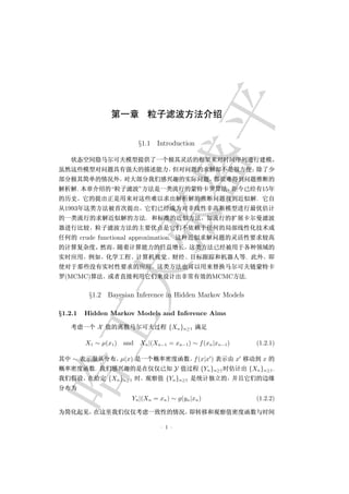
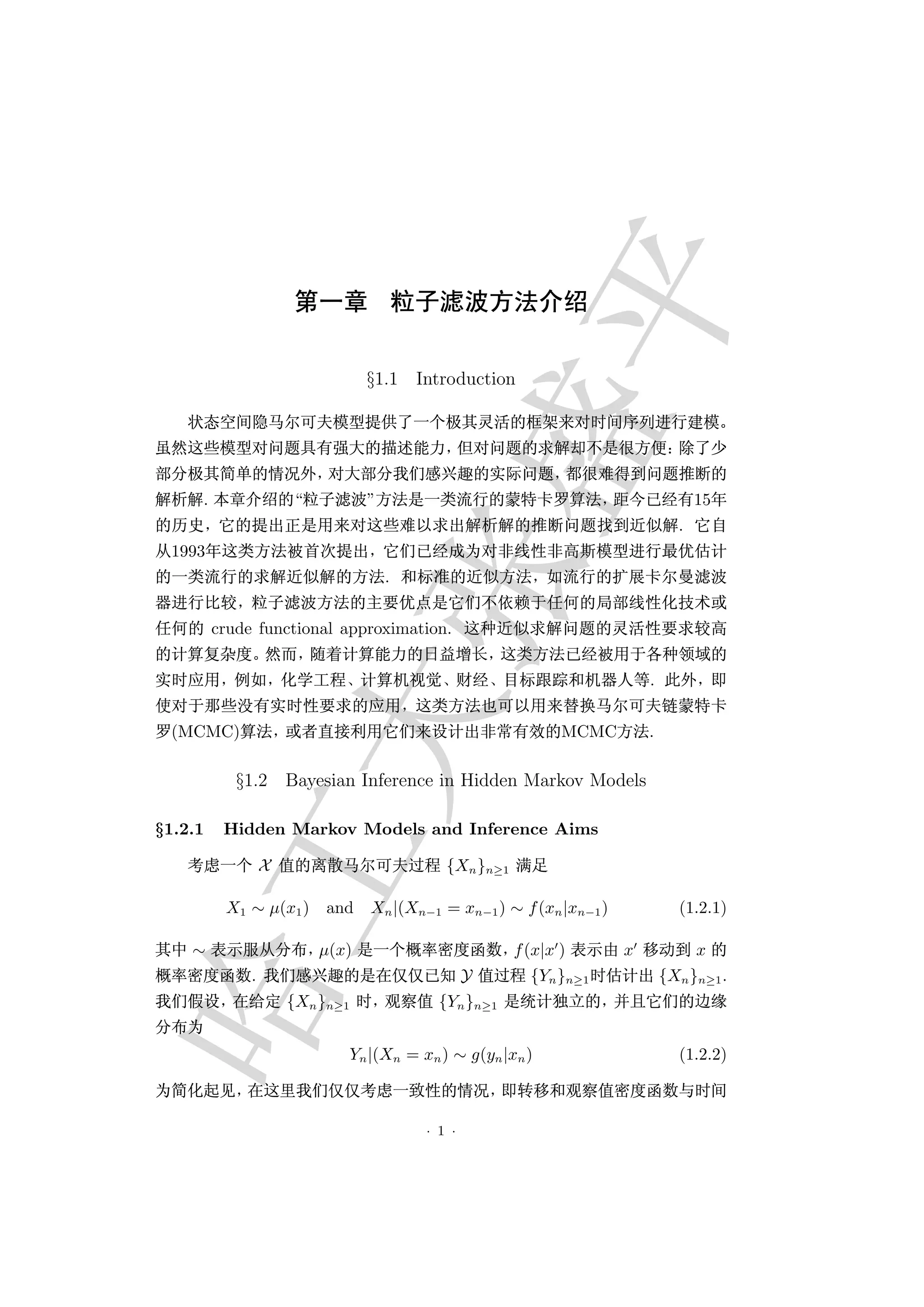
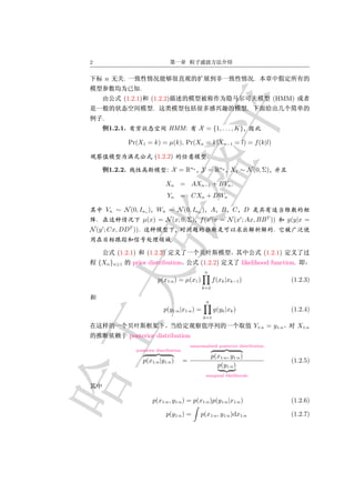
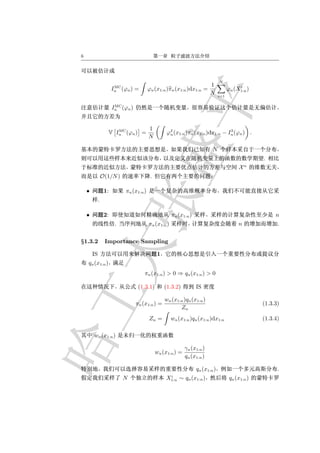
1) Bayesian inference in hidden Markov models aims to compute the posterior distribution p(x1:n|y1:n) and marginal likelihoods p(y1:n) given observed data y1:n. This can be done using filtering recursions to calculate the marginal distributions p(xn|y1:n) and likelihoods p(y1:n). 2) Sequential Monte Carlo (SMC) methods, also known as particle filters, provide a way to approximate the filtering distributions and likelihoods using a set of random samples or "particles". Importance sampling is used to assign importance weights to the particles to represent the target distributions. 3) Sequential importance sampling (SIS) recursively propag

1. §1.1 Introduction
. “ ” 15
.
1993
.
crude functional approximation.
.
(MCMC) MCMC .
§1.2 Bayesian Inference in Hidden Markov Models
§1.2.1 Hidden Markov Models and Inference Aims
X {Xn }n≥1
X1 ∼ µ(x1 ) and Xn |(Xn−1 = xn−1 ) ∼ f (xn |xn−1 ) (1.2.1)
∼ µ(x) f (x|x ) x x
. Y {Yn }n≥1 {Xn }n≥1 .
{Xn }n≥1 {Yn }n≥1
Yn |(Xn = xn ) ∼ g(yn |xn ) (1.2.2)
· 1 ·

2. 2
n . .
.
(1.2.1) (1.2.2) (HMM)
. .
.
1.2.1. HMM X = {1, . . . , K}
Pr(X1 = k) = µ(k), Pr(Xn = k|Xn−1 = l) = f (k|l)
(1.2.2) .
1.2.2. X = Rnx Y = Rny X1 ∼ N (0, Σ)
Xn = AXn−1 + BVn ,
Yn = CXn + DWn
Vn ∼ N (0, Inv ) Wn ∼ N (0, Inw ) A B C D
. µ(x) = N (x; 0, Σ) f (x |x = N (x ; Ax, BB T )) g(y|x =
T
N (y ; Cx, DD )). .
.
(1.2.1) (1.2.2) (1.2.1)
{Xn }n≥1 prior distribution (1.2.2) likelihood function.
n
p(x1:n ) = µ(x1 ) f (xk |xk−1 ) (1.2.3)
k=2
n
p(y1:n |x1:n ) = g(yk |xk ) (1.2.4)
k=1
Y1:n = y1:n X1:n
posterior distribution
unnormalised posterior distribution
posterior distribution
p(x1:n , y1:n )
p(x1:n |y1:n ) = (1.2.5)
p(y1:n )
marginal likelihoods
p(x1:n , y1:n ) = p(x1:n )p(y1:n |x1:n ) (1.2.6)
p(y1:n ) = p(x1:n , y1:n )dx1:n (1.2.7)

3. §1.2 Bayesian Inference in Hidden Markov Models 3
(1.2.5) (1.2.6)
( (1.2.3) (1.2.4)). (1.2.7) .
1.2.1 (1.2.7)
(1.2.5)
. 1.2.2 p(x1:n |y1:n )
.
.
p(x1:n |y1:n ) p(y1:n ).
.
• Filtering and Marginal likelihood computation
posterior distribution {p(x1:n |y1:n )}n≥1 marginal likelihoods
{p(y1:n )}n≥1 . p(x1 |y1 ) p(y1 )
p(x1:2 |y1:2 ) p(y1:2 ) .
. marginal distributions
{p(xn |y1:n )}n≥1 {p(x1:n |y1:n )}n≥1 .
• Smoothing: p(x1:T |y1:T )
{p(xn |y1:T )} n = 1, . . . , T .
§1.2.2 Filtering and Marginal Likelihood
.
.
{Y1:n = y1:n } X1:n Xn .
posterior distribution p(x1:n |y1:n ) (1.2.5) prior distribution
p(x1:n ) (1.2.3) likelihood function (1.2.4) . (1.2.5)
unnormalised posterior distribution p(x1:n , y1:n )
p(x1:n , y1:n ) = p(x1:n−1 , y1:n−1 )p(xn , yn |x1:n−1 , y1:n−1 )
= p(x1:n−1 , y1:n−1 )p(xn |xn−1 )p(yn |xn ) (1.2.8)
= p(x1:n−1 , y1:n−1 )f (xn |xn−1 )g(yn |xn )

4. 4
posterior p(x1:n |y1:n )
p(x1:n , y1:n )
p(x1:n |y1:n ) =
p1:n
p(x1:n−1 , y1:n−1 )f (xn |xn−1 )g(yn |xn )
= (1.2.9)
p(y1:n−1 )p(yn |yn−1 )
f (xn |xn−1 )g(yn |xn )
= p(x1:n−1 |y1:n−1 )
p(yn |y1:n−1 )
p(yn |y1:n−1 ) = p(yn , xn−1:n |y1:n−1 )dxn−1:n
= p(xn−1 |y1:n−1 )p(yn , xn |xn−1 , y1:n−1 )dxn−1:n (1.2.10)
= p(xn−1 |y1:n−1 )f (xn |xn−1 )g(yn |xn )dxn−1:n
(1.2.10) .
.
(1.2.9) x1:n−1 marginal distribution p(xn |y1:n )
g(yn |xn )p(xn |y1:n−1 )
p(xn |y1:n ) = (1.2.11)
p(yn |y1:n−1 )
p(xn |y1:n−1 ) = f (xn |xn−1 )p(xn−1 |y1:n−1 )dxn−1 (1.2.12)
(1.2.12) (1.2.11) .
(1.2.9) (1.2.11) (1.2.12).
{p(x1:n |y1:n )} {p(xn |y1:n )}
marginal likelihood p(y1:n )
n
p(y1:n ) = p(y1 ) p(yk |y1:k−1 ) (1.2.13)
k=2
p(yk |y1:k−1 ) (1.2.10) .
§1.2.3 Summary
.
1.2.1 1.2.2 .
.
N .
( N →∞ ).

5. §1.3 Sequential Monte Carlo Methods 5
§1.3 Sequential Monte Carlo Methods
15 SMC
. SMC
. SMC . SMC
{πn (x1:n )} . πn (x1:n )
n
X .
γn (x1:n )
πn (x1:n ) = (1.3.1)
Zn
γn : X n → R+
Zn = γn (x1:n )dx1:n (1.3.2)
. SMC 1 π1 (x1 ) Z1
2 π2 (x1:2 ) Z2 .
γn (x1:n ) = p(x1:n , y1:n ) Zn = p(y1:n ) πn (x1:n ) =
p(x1:n |y1:n ).
§1.3.1 Basics of Monte Carlo Methods
n πn (x1:n ).
i
N X1:n ∼ πn (x1:n ) πn (x1:n )
N
1
πn (x1:n ) =
ˆ δX1:n (x1:n )
i
N i=1
δx0 (x) x0 Dirac delta mass.
+∞, x = x0
δx0 (x) =
0, x = x0
+∞
δx0 (x)dx = 1.
−∞
πn (xk )
N
1
πn (xk ) =
ˆ δXk (xk )
i
N i=1
ϕn : X n → R
In (ϕn ) = ϕn (x1:n )πn (x1:n )dx1:n

6. 6
N
MC 1 i
In (ϕn ) = ϕn (x1:n )πn (x1:n )dx1:n = ϕn (X1:n )
N i=1
MC
In (ϕn )
MC 1
V In (ϕn ) = ϕ2 (x1:n )πn (x1:n )dx1:n − In (ϕn ) .
n
2
N
N
.
n
X
O(1/N ) .
• 1: πn (x1:n )
.
• 2: πn (x1:n ) n
. πn (x1:n ) n .
§1.3.2 Importance Sampling
IS 1
qn (x1:n )
πn (x1:n ) > 0 ⇒ qn (x1:n ) > 0
(1.3.1) (1.3.2) IS
wn (x1:n )qn (x1:n )
πn (x1:n ) = (1.3.3)
Zn
Zn = wn (x1:n )qn (x1:n )dx1:n (1.3.4)
wn (x1:n )
γn (x1:n )
wn (x1:n ) =
qn (x1:n )
qn (x1:n ) .
i
N X1:n ∼ qn (x1:n ) qn (x1:n )

7. §1.3 Sequential Monte Carlo Methods 7
(1.3.3) (1.3.4)
n
i
πn (x1:n ) = Wn δX1:n (x1:n )
i (1.3.5)
i=1
N
1 i
Zn = wn (X1:n ) (1.3.6)
N i=1
i
i wn (X1:n )
Wn = n j (1.3.7)
j=1 wn (X1:n )
In (ϕn )
N
IS i i
In (ϕn ) = ϕn (x1:n )πn (x1:n )dx1:n = Wn ϕn (X1:n )
i=1
§1.3.3 Sequential Importance Sampling
2 n
.
qn (x1:n ) = qn−1 (x1:n−1 )qn (xn |x1:n−1 )
n
= q1 (x1 ) qk (xk |x1:k−1 ) (1.3.8)
k=2
i
n X1:n ∼ qn (x1:n )
i i i
1 X1 ∼ q1 (x1 ) k = 2, . . . , n Xk ∼ qk (xk |X1:k−1 ).
γn (x1:n )
wn (x1:n ) =
qn (x1:n )
γn−1 (x1:n−1 ) γn (x1:n )
= (1.3.9)
qn−1 (x1:n−1 ) γn−1 (x1:n−1 )qn (xn |x1:n−1 )
wn (x1:n ) = wn−1 (x1:n−1 ) · αn (x1:n )
n
= w1 (x1 ) αk (x1:k ) (1.3.10)
k=2
incremental importance weight αn (x1:n )
γn (x1:n )
αn (x1:n ) = . (1.3.11)
γn−1 (x1:n−1 )qn (xn |x1:n−1 )

8. 8
SIS :
Algorithm 1: Sequential Importance Sampling
1 n=1
2 for i = 1 to N do
i
3 X1 ∼ q1 (x1 )
i i i
4 w1 (X1 ) W1 ∝ w1 (X1 )
5 end
6 for n = 2 to T do
7 for i = 1 to N do
i i
8 Xn ∼ qn (xn |X1:n−1 )
9
i i i
wn (X1:n ) = wn−1 (X1:n−1 ) · αn (X1:n ),
i i
Wn ∝ wn (X1:n ).
10 end
11 end
n πn (x1:n ) Zn πn (x1:n ) (1.3.5) Zn
(1.3.6). Zn /Zn−1
N
Zn i i
= Wn−1 αn X1:n .
Zn−1 i=1
SIS n qn (xn |x1:n−1 ).
wn (x1:n ) .
opt
qn (xn |x1:n−1 ) = πn (xn |x1:n−1 )
x1:n−1 wn (x1:n ) incremental weight
opt γn (x1:n−1 ) γn (x1:n )dxn
αn (x1:n ) = = .
γn−1 (xn−1 ) γn−1 (x1:n−1 )
opt
πn (xn |x1:n−1 ) αn (x1:n ).
opt
qn (xn |x1:n−1 ) .
qn qn (xn |x1:n−1 )
αn (x1:n ) n 2. SIS
. IS n
. SIS IS
(1.3.8) SIS .
.

9. §1.3 Sequential Monte Carlo Methods 9
1.3.1. X =R
n n
πn (x1:n ) = πn (xk ) = N (xk ; 0, 1), (1.3.12)
k=1 k=1
n
x2
k
γn (x1:n ) = exp − ,
k=1
2
Zn = (2π)n/2 .
n n
qn (x1:n ) = qk (xk ) = N (xk ; 0, σ 2 ).
k=1 k=1
1
σ2 > 2
VIS Zn < ∞ relative variance
VIS Zn 1 σ4
n/2
= −1 .
2
Zn N 2σ 2 − 1
1 σ4
σ 2
< σ2 = 1 2σ 2 −1
>1 relative variance
n . σ = 1.2
VIS [Zn ] VIS [Zn ]
qk (xk ) ≈ πn (xk ) N 2
Zn
≈ (1.103)n/2 . n = 1000 N 2
Zn
≈
21 23
1.9 × 10 N ≈ 2 × 10 relative variance
VIS [Zn ]
Z2
= 0.01 .
n
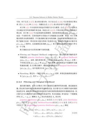
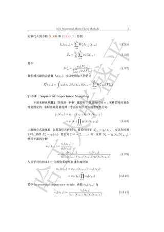
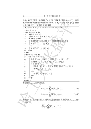
§1.3.4 Resampling
IS SIS n
SMC .
. πn (x1:n ) IS
πn (x1:n ) qn (x1:n )
πn (x1:n ) . πn (x1:n )
i i
IS πn (x1:n ) Wn X1:n
resampling πn (x1:n )
. πn (x1:n ) N
i i
πn (x1:n ) N X1:n Nn
1:N 1 N 1:N
Nn = (Nn , . . . , Nn ) (N, Wn )
1/N . resampled empirical measure
πn (x1:n )
N i
Nn
π n (x1:n ) = δX i (x1:n ) (1.3.13)
i=1
N 1:n

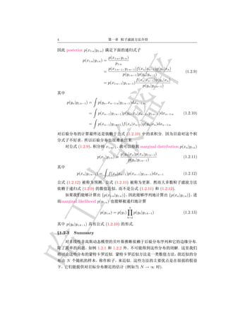
10. 10
i 1:N i
E [Nn |Wn ] = N Wn . π n (x1:n ) πn (x1:n ) .
1
• Systematic Resampling U1 ∼ U 0, N i = 2, . . . , N
i−1 i i−1 k i k
Ui = U1 + N
Nn = Uj : k=1 Wn ≤ Uj ≤ k=1 Wn
0
k=1 = 0.
i i 1:N
• Residual Resampling Nn = N W n N, W n
1:N i i
Nn W n ∝ Wn − N −1 Nn
i i i i
Nn = Nn + N n .
1:N 1:N
• Multinomial Resampling (N, Wn ) Nn .
O(N ) . systematic
resampling
.
πn (x1:n )
In (ϕn ) πn (x1:n )
π n (x1:n ) .
.
.
n n+1
.
. .
§1.3.5 A Generic Sequential Monte Carlo Algorithm
SMC SIS . 1
i i
π1 (x1 ) IS π1 (x1 ) {W1 , X1 }.
.
1 i i
{ N , X 1} . X1
i i j1 j2
N1 N1 j1 = j2 = · · · = jN1
i X1 = X1 =
jN i i
i i
· · · = X1 1
= X1 . SIS X2 ∼ q2 (x2 |X 1 ).
i i
(X 1 , X2 ) π1 (x1 )q2 (x2 |x1 ).
incremental weights α2 (x1:2 ).

11. §1.3 Sequential Monte Carlo Methods 11
. :
Algorithm 2: Sequential Monte Carlo
1 n=1
2 for i = 1 to N do
i
3 X1 ∼ q1 (x1 )
i i i
4 w1 (X1 ) W1 ∝ w1 (X1 )
i i 1 i
5 {W1 , X1 } N { N , X 1}
6 end
7 for n = 2 to T do
8 for i = 1 to N do
i i i i i
9 Xn ∼ qn (xn |X 1:n−1 ) X1:n ← X 1:n−1 , Xn
i i i
10 αn (X1:n ) Wn ∝ αn (X1:n )
i i 1 i
11 {Wn , X1:n } N { N , X 1:n }
12 end
13 end
n πn (x1:n ) . :
N
i
πn (x1:n ) = Wn δX1:n (x1:n )
i (1.3.14)
i=1
N
1 i
π n (x1:n ) = Wn δX i (x1:n ) (1.3.15)
N i=1
1:n
(1.3.14) (1.3.15) . Zn /Zn−1
N
Zn 1 i
= αn X1:n
Zn−1 N i=1
.
.
.
Effective Sample Size (ESS)
. n ESS
N −1
i
ESS = Wn .
i=1
N (
) ESS . ESS 1 N

12. 12
NT . NT = N/2.
i 1 i
. Wn = N
{Wn }
. .
Algorithm 3: Sequential Monte Carlo with Adaptive Resampling
1 n=1
2 for i = 1 to N do
i
3 X1 ∼ q1 (x1 )
i i i
4 w1 (X1 ) W1 ∝ w1 (X1 )
5 if then
i i 1 i
6 {W1 , X1 } N { N , X 1}
i i 1 i
7 {W 1 , X 1 } ← { N , X 1 }
8 else
i i i i
9 {W 1 , X 1 } ← {W1 , X1 }
10 end
11 end
12 for n = 2 to T do
13 for i = 1 to N do
i i i ii
14 Xn ∼ qn (xn |X 1:n−1 ) X1:n ← (X 1:n−1 , Xn
i i i i
15 αn (X1:n ) Wn ∝ W n−1 αn (X1:n )
16 if then
i i 1 i
17 {Wn , X1:n } N { N , X 1:n }
i i 1 i
18 {W n , X n } ← { N , X n }
19 else
i i i i
20 {W 1 , X 1 } ← {Wn , Xn }
21 end
22 end
23 end
πn (x1:n ) .
N
i
πn (x1:n ) = Wn δX1:n (x1:n ),
i (1.3.16)
i=1
N
i
π n (x1:n ) = W n δX i (x1:n ) (1.3.17)
1:n
i=1
n . Zn /Zn−1
N
Zn i i
= W n−1 αn X1:n
Zn−1 i=1

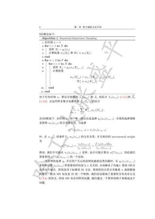
13. §1.4 Particle Filter 13
1
1.3.1 σ2 > 2
asymptotic variance
VSMC Zn n σ4
1/2
= −1
2
Zn N 2σ 2 − 1
VIS Zn 1 σ4
n/2
= −1 .
2
Zn N 2σ 2 − 1
SMC n IS n
2
. σ = 1.2 qk (xk ) ≈ πn (xk ).
n = 1000 IS N ≈ 2 × 1023
VIS [Zn ] VSMC [Zn ]
Zn 2 = 10−2 . 2
Zn
= 10−2 SMC
N ≈ 104 19 .
§1.3.6 Summary
SMC {πn (x1:n )} {Zn }.
• n qn (xn |x1:n−1 )
αn (x1:n ) n .
• k n > k πn (x1:k )
SMC . n
{πn (x1:n )} SMC . , πn (x1 )
.
§1.4 Particle Filter
SMC SIS
.
{p(x1:n |y1:n )}n≥1 .
ESS .
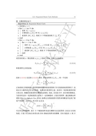
§1.4.1 SMC for Filtering
SMC {p(x1:n |y1:n )}n≥1

14. 14
πn (x1:n ) = p(x1:n |y1:n )
γ( x1:n ) = p(x1:n , y1:n )
Zn = p(y1:n ) (1.4.1)
nonumber (1.4.2)
qn (x1:n ) qn (xn |x1:n−1 ).
IS qn (x1:n ) SIS
qn (xn |x1:n−1 ) .
n
opt
qn (xn |x1:n−1 ) = πn (xn |x1:n−1Z )
= p(xn |yn , xn−1 )
g(yn |xn )f (xn |xn−1 )
= (1.4.3)
p(yn |xn−1 )
incremental importance weight
αn (x1:n ) = p(yn |xn−1 )
opt
qn (xn |x1:n−1 )
qn (xn |x1:n−1 ) = q(xn |yn , xn−1 ) (1.4.4)
(1.3.9) (1.3.11) (1.4.4) incremental weight
g(yn |xn )f (xn |xn−1 )
αn (x1:n ) = αn (xn−1:n ) = .
q(xn |yn , xn−1 )

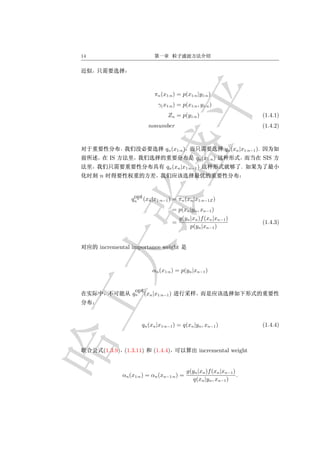
15. §1.4 Particle Filter 15
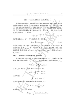
Algorithm 4: SMC for Filtering
1 n=1
2 for i = 1 to N do
i
3 X1 ∼ q1 (x1 |y1 )
i µ(xi )g(y1 |X1 )
i
i i
4 w1 (X1 ) = 1
i
q(Xi |y1 )
W1 ∝ w1 (X1 )
i i 1 i
5 {W1 , X1 } N { N , X 1}
6 end
7 for n = 2 to T do
8 for i = 1 to N do
i i i i i
9 Xn ∼ qn (xn |yn , X n−1 ) X1:n ← (X 1:n−1 , Xn )
i i i
i g(yn |Xn )f (Xn |Xn−1 ) i i
10 αn (Xn−1:n ) = i i
q(Xn |yn ,Xn−1 )
Wn ∝ αn (Xn−1:n )
i i 1 i
11 {Wn , X1:n } N { N , X 1:n }
12 end
13 end
[1] A.D. and A. Johansen, Particle filtering and smoothing: Fifteen years later, in Hand-
book of Nonlinear Filtering (eds. D. Crisan et B. Rozovsky), Oxford University Press,
2009. See http://www.cs.ubc.ca/~arnaud