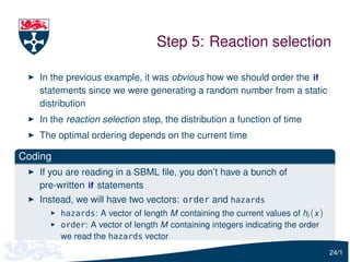
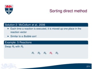
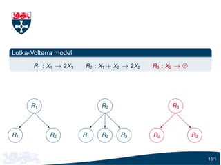
Unraveling Multimodality with Large Language Models.pdf
Speeding up the Gillespie algorithm
1. Speeding up the Gillespie algorithm
Colin Gillespie
School of Mathematics & Statistics
2. Outline
1. Brief description of stochastic kinetic models
2. Gillespie’s direct method
Different Gillespie!
3. Discussion
2/1
3. Stochastic kinetic models
Suppose we have:
N species: X1 , X2 , . . . , XN
M reactions: R1 , R2 , . . . , RM
In a “typical” model, M = 3N.
Reaction Ri takes the form
ci
Ri : ui1 X1 + . . . + uik XN −→ vi1 X1 + . . . + vik XN .
−
The effect of reaction i on species j is to change Xj by an amount vij − uij .
3/1
4. Mass action kinetics
Example zeroth-order reaction: if reaction Ri has the form
ci
Ri : ∅ − Xk
→
then the rate that this reaction occurs is
hi (x ) = ci .
The effect of this reaction is
xk = xk + 1 .
4/1
5. Mass action kinetics
Example first-order reaction: if reaction Ri has the form
ci
Ri : Xj − 2Xj
→
then the rate that this reaction occurs is
hi (x ) = ci xj
where xj is the number of molecules of Xj at time t. The effect of this
reaction is
xj = xj + 1 .
5/1
6. Mass action kinetics
Example second-order reaction: if reaction Ri has the form
ci
Ri : Xj + Xk − Xk
→
then the rate that this reaction occurs is
hi (x ) = ci xj xk .
The effect of this reaction is
xj = xj − 1
There is no overall effect on Xk . For example, Xk could be an enzyme.
6/1
7. Lotka-Volterra model
R1 : X1 → 2X1 R2 : X1 + X2 → 2X2 R3 : X2 → ∅
So R1 and R3 are first-order reactions and R2 is a second order reaction.
7/1
8. The Gillespie algorithm
(Dan) Gillespie has developed a number of algorithms. The “Gillespie
algorithm” refers to his 1977 Journal of Chemical Physics paper (cited
∼ 1800 times)
Kendall’s 1950’s paper “An artificial realisation of a simple birth and
death process”, simulated a simple model using a table of random
numbers (cited ∼ not very often)
8/1
9. The Gillespie algorithm
(Dan) Gillespie has developed a number of algorithms. The “Gillespie
algorithm” refers to his 1977 Journal of Chemical Physics paper (cited
∼ 1800 times)
Kendall’s 1950’s paper “An artificial realisation of a simple birth and
death process”, simulated a simple model using a table of random
numbers (cited ∼ not very often)
8/1
11. The direct method
1. Initialisation: initial conditions, reactions constants, and random
number generators
2. Propensities update: Update each of the M hazard functions, hi (x )
3. Propensities total: Calculate the total hazard h0 = ∑M 1 hi (x )
i=
4. Reaction time: τ = −ln [U (0, 1)]/h0 and t = t + τ
5. Reaction selection: A reaction is chosen proportional to it’s hazard
6. Reaction execution: Update species
7. Iteration: If the simulation time is exceeded stop, otherwise go back
to step 2
Typically there are a large number of iterates.
10/1
12. The Gillespie slow down
As the number of reactions (and species) increase, the length of time a
single iteration takes also increases
Example
In the next few slides we will consider a toy model:
ci
Xi − ∅,
→ i=1, . . . , N
where N = M = 600, xi (0) = 1000, ci = 1 and the final time is T = 30.
So
hi (x ) = ci xi
11/1
13. The Gillespie algorithm
When we discuss this algorithm we are thinking about software which
reads in a description of your model in SBML (say), and runs
stochastic simulations
Examples: Copasi, celldesigner, gillespie2
12/1
14. Step 2: Propensities update
At each iteration we update each of the M hazards. That is we
calculate hi (x ) for i = 1, . . . , M. This is O (M )
However, after a single reaction has occurred we actually only need
to update the hazards that have changed
Toy Example
If reaction 1 occurs
c1
R1 : X1 − ∅,
→
only species X1 is changed
The only hazard that contains X1 is R1
13/1
15. Step 2: Propensities update
At each iteration we update each of the M hazards. That is we
calculate hi (x ) for i = 1, . . . , M. This is O (M )
However, after a single reaction has occurred we actually only need
to update the hazards that have changed
Toy Example
If reaction 1 occurs
c1
R1 : X1 − ∅,
→
only species X1 is changed
The only hazard that contains X1 is R1
13/1
16. Dependency graphs
Construct a dependency graph for the hazards
For the toy model the graph just contains M = 600 independent
nodes
R1 R2 r r r r r RM
14/1
25. Dependency graph
So instead of updating all M reactions, we only need to update D
propensities. Usually D 6
However, constructing and traversing the graph also takes time
So we would only implement this data structure if M 10
17/1
26. Step 3: Propensities total
At each iteration we combine all M hazards - O (M )
M
h0 ( x ) = ∑ hi (x ) .
i =1
However, after a single reaction has occurred we only need to update
the hazards that have change
If we have used a dependency graph for the reaction network then
we can subtract the old hazard values from h0
add the new hazards values to h0
18/1
27. Step 3: Propensities total
At each iteration we combine all M hazards - O (M )
M
h0 ( x ) = ∑ hi (x ) .
i =1
However, after a single reaction has occurred we only need to update
the hazards that have change
If we have used a dependency graph for the reaction network then
we can subtract the old hazard values from h0
add the new hazards values to h0
18/1
28. Step 3: Propensities total
Toy model
If reaction Ri fires, then
new old
h0 = h0 − hiold + hinew
One addition and a one subtraction instead of 600 additions
19/1
29. Step 4: Reaction time
Reaction time: τ = −ln [U (0, 1)]/h0 . As the number of reactions and
species increase, the time of this step is constant.
For the toy model, we spend about 3% of computer time executing
this step
You could generate the random numbers on a separate thread (on a
multicore machines) to save you a small amount of time
20/1
30. Step 5: Reaction selection
We choose a reaction proportional to it’s propensity. Or search for the
µ that satisfies this equation:
µ µ −1
∑ hi ( x ) U × h0 ( x ) ∑ hi ( x ) ,
i =1 i =1
where U ∼ U (0, 1)
This is O (M )
The key to reducing this bottleneck is noting that in most systems,
some reactions occur more often than others. The model system is
multi-scale.
To speed up this step, we order the hi ’s in terms of size
21/1
31. Step 5: Reaction selection
We choose a reaction proportional to it’s propensity. Or search for the
µ that satisfies this equation:
µ µ −1
∑ hi ( x ) U × h0 ( x ) ∑ hi ( x ) ,
i =1 i =1
where U ∼ U (0, 1)
This is O (M )
The key to reducing this bottleneck is noting that in most systems,
some reactions occur more often than others. The model system is
multi-scale.
To speed up this step, we order the hi ’s in terms of size
21/1
32. Step 5: Reaction selection
Consider the following pieces of R code:
}
## u are U(0, 1) RNs
for (i in 1: length (u)) {
i f (u[i] 0.01)
x = 1
else i f (u[i]0.05)
x = 2
else i f (u[i]0.1)
x = 3
else
x = 4
Calling this piece of code 107 times takes about 34 seconds.
22/1
33. Step 5: Reaction selection
Now lets just reverse the order of the if statements
}
for (i in 1: length (u)) {
i f (u[i] 0.9)
x = 1
else i f (u[i]0.95)
x = 2
else i f (u[i]0.99)
x = 3
else
x = 4
Calling this piece of code 107 times takes about 15 seconds. A reduction
of around 44%.
23/1
34. Step 5: Reaction selection
In the previous example, it was obvious how we should order the if
statements since we were generating a random number from a static
distribution
In the reaction selection step, the distribution a function of time
The optimal ordering depends on the current time
Coding
If you are reading in a SBML file, you don’t have a bunch of
pre-written if statements
Instead, we will have two vectors: order and hazards
hazards: A vector of length M containing the current values of hi (x )
order: A vector of length M containing integers indicating the order
we read the hazards vector
24/1
35. Step 5: Reaction selection
In the previous example, it was obvious how we should order the if
statements since we were generating a random number from a static
distribution
In the reaction selection step, the distribution a function of time
The optimal ordering depends on the current time
Coding
If you are reading in a SBML file, you don’t have a bunch of
pre-written if statements
Instead, we will have two vectors: order and hazards
hazards: A vector of length M containing the current values of hi (x )
order: A vector of length M containing integers indicating the order
we read the hazards vector
24/1
40. Optimised direct method
Solution 1 - Cao et al., 2004
Run a few presimulations for a short period of time t max-time
Reorder your hazard vector according to the presimulations
Run your main simulation
26/1
41. Optimised direct method
Solution 1 - Cao et al., 2004
Run a few presimulations for a short period of time t max-time
Reorder your hazard vector according to the presimulations
Run your main simulation
Lotka-Volterra
Using the standard parameters from Boys, Wilkinson Kirkwood,
in a typical simulation, reactions R1 , R2 and R3 occur in roughly
equal amounts.
26/1
42. Optimised direct method
Solution 1 - Cao et al., 2004
Run a few presimulations for a short period of time t max-time
Reorder your hazard vector according to the presimulations
Run your main simulation
Disadvantages
Clearly doing presimulations isn’t great
How long should you simulate for?
Presimulations will be time consuming
The order of reactions is fixed. So at some simulations points
the order may be sub-optimal.
26/1
43. Sorting direct method
Solution 2: McCollum et al., 2006
Each time a reaction is executed, it is moved up one place in the
reaction vector
Similar to a Bubble sort
Example: 5 Reactions
27/1
44. Sorting direct method
Solution 2: McCollum et al., 2006
Each time a reaction is executed, it is moved up one place in the
reaction vector
Similar to a Bubble sort
Example: 5 Reactions
Execute R4
R1 R2 R3 R4 R5
27/1
45. Sorting direct method
Solution 2: McCollum et al., 2006
Each time a reaction is executed, it is moved up one place in the
reaction vector
Similar to a Bubble sort
Example: 5 Reactions
Swap R4 with R3
R1 R2 R4 R3 R5
27/1
46. Sorting direct method
Solution 2: McCollum et al., 2006
Each time a reaction is executed, it is moved up one place in the
reaction vector
Similar to a Bubble sort
Example: 5 Reactions
Execute R5
R1 R2 R4 R3 R5
27/1
47. Sorting direct method
Solution 2: McCollum et al., 2006
Each time a reaction is executed, it is moved up one place in the
reaction vector
Similar to a Bubble sort
Example: 5 Reactions
Swap R5 with R3
R1 R2 R4 R5 R3
27/1
48. Sorting direct method
Solution 2: McCollum et al., 2006
Each time a reaction is executed, it is moved up one place in the
reaction vector
Similar to a Bubble sort
Example: 5 Reactions
Execute R4
R1 R2 R4 R5 R3
27/1
49. Sorting direct method
Solution 2: McCollum et al., 2006
Each time a reaction is executed, it is moved up one place in the
reaction vector
Similar to a Bubble sort
Example: 5 Reactions
Swap R4 with R2
R1 R4 R2 R5 R3
27/1
50. Sorting direct method
Solution 2: McCollum et al., 2006
Each time a reaction is executed, it is moved up one place in the
reaction vector
Similar to a Bubble sort
Example: 5 Reactions
Execute R5
R1 R4 R2 R5 R3
27/1
51. Sorting direct method
Solution 2: McCollum et al., 2006
Each time a reaction is executed, it is moved up one place in the
reaction vector
Similar to a Bubble sort
Example: 5 Reactions
Swap R5 with R2
R1 R4 R5 R2 R3
27/1
52. Sorting direct method
Solution 2: McCollum et al., 2006
The swapping effectively reduces the search depth for a reaction the
next time it’s executed
Only requires a swap of two memory addresses, so very little
overhead
Handles sharp changes in propensity, such as on/off behaviour in
switches
Easy to code
Reduces the problem to order O (S), where S is the search distance
28/1
53. Binary searches
Binary search Li Petzold, Tech Report. 2006
Composition and Rejection scheme - Slepoy et al. J. Chem. Phys.
2008
I suspect these methods are only useful for very large systems
29/1
54. Binary searches
Binary search Li Petzold, Tech Report. 2006
Composition and Rejection scheme - Slepoy et al. J. Chem. Phys.
2008
I suspect these methods are only useful for very large systems
0.12
0.10
0.08
0.06
0.04
0.02
0.00
Reactions
29/1
55. Binary searches
Binary search Li Petzold, Tech Report. 2006
Composition and Rejection scheme - Slepoy et al. J. Chem. Phys.
2008
I suspect these methods are only useful for very large systems
0.12
0.6
0.10
0.4
0.08
0.06
0.04
0.02
0.00
Reactions
29/1
56. Binary searches
Binary search Li Petzold, Tech Report. 2006
Composition and Rejection scheme - Slepoy et al. J. Chem. Phys.
2008
I suspect these methods are only useful for very large systems
0.12
0.10
0.08
0.06
0.04
0.02
0.00
Reactions
29/1
57. Binary searches
Binary search Li Petzold, Tech Report. 2006
Composition and Rejection scheme - Slepoy et al. J. Chem. Phys.
2008
I suspect these methods are only useful for very large systems
0.12
0.10
0.08
0.06
0.04
0.02
0.00
Reactions
29/1
58. Binary searches
Binary search Li Petzold, Tech Report. 2006
Composition and Rejection scheme - Slepoy et al. J. Chem. Phys.
2008
I suspect these methods are only useful for very large systems
0.12
0.10
0.08
0.06
0.04
0.02
0.00
Reactions
29/1
59. Binary searches
Binary search Li Petzold, Tech Report. 2006
Composition and Rejection scheme - Slepoy et al. J. Chem. Phys.
2008
I suspect these methods are only useful for very large systems
29/1
60. Step 6: Reaction execution
After a reaction has fired, update the species
Naively, we could update all species after a reaction has fired
x = x + S (j )
where S (j ) = v (j ) − u (j ) denotes the j th column of the stoichiometry
matrix S. This operation would be O (N )
However, S is almost certainly sparse. In the toy model, we have:
R1 : X1 → ∅
so
S (1) = (−1, 0, 0, 0, . . . , 0, 0, 0)
30/1
61. Step 6: Reaction execution
After a reaction has fired, update the species
Naively, we could update all species after a reaction has fired
x = x + S (j )
where S (j ) = v (j ) − u (j ) denotes the j th column of the stoichiometry
matrix S. This operation would be O (N )
However, S is almost certainly sparse. In the toy model, we have:
R1 : X1 → ∅
so
S (1) = (−1, 0, 0, 0, . . . , 0, 0, 0)
30/1
62. Sparse vectors
Instead we use compressed column format for storage
For each column in the stoichiometry matrix we have two vectors:
1. A vector of the non-zero values
2. A vector of indices for the non-zero values
31/1
63. Sparse vectors
Instead we use compressed column format for storage
For each column in the stoichiometry matrix we have two vectors:
1. A vector of the non-zero values
2. A vector of indices for the non-zero values
Toy model
So
S (1) = (−1, 0, 0, 0, . . . , 0, 0, 0)
would be represented as:
V1 = (−1) and C1 = (1)
31/1
64. Lotka-Volterra system
For the Lotka-Volterra reaction:
R2 : X1 + X2 → 2X2
we have the stoichiometry matrix column:
S (2) = (−1, 1)
which would be represented as:
V2 = (−1, 1) and C2 = (1, 2)
32/1
65. Lotka-Volterra system
For the Lotka-Volterra reaction:
R2 : X1 + X2 → 2X2
we have the stoichiometry matrix column:
S (2) = (−1, 1)
which would be represented as:
V2 = (−1, 1) and C2 = (1, 2)
32/1
66. Discussion
The Gillespie algorithm is a fairly easy method to implement, but we
can achieve impressive increases of execution speed with efficient
data structures
In fact “clever programming” can turn an obviously slow algorithm into
a faster, more efficient method
Gibson-Bruck did this with Gillespie’s first reaction method
Topic of my next talk
33/1
67. Discussion
This highlights that it can be very difficult to carry out speed
comparisons of different algorithms.
What do we mean when we measure the speed of an algorithm?
We need to be sure that the slowness of an algorithm isn’t down to bad
programming
Likelihood free techniques require millions of simulator calls. It is
crucial that you have an efficient simulator.
34/1
68. Discussion
This highlights that it can be very difficult to carry out speed
comparisons of different algorithms.
What do we mean when we measure the speed of an algorithm?
We need to be sure that the slowness of an algorithm isn’t down to bad
programming
Likelihood free techniques require millions of simulator calls. It is
crucial that you have an efficient simulator.
However,
“....premature optimisation is the root of all evil”
Donald Knuth
34/1
69. Further Reading
Gillespie, D., 1977. Exact Stochastic Simulation of Coupled Chemical Reactions. The Journal of Physical Chemistry.
Kendall, D. G., 1950. An artificial realisation of a simple birth and death process. Journal of the Royal Statistical Society, B.
McCollum JM, Peterson GD, Cox CD, Simpson ML, Samatova NF., 2006. The sorting direct method for stochastic simulation of
biochemical systems with varying reaction execution behavior. Computational Biology and Chemistry.
Slepoy A, Thompson AP, Plimpton SJ., 2008. A constant-time kinetic Monte Carlo algorithm for simulation of large biochemical
reaction networks. The Journal of Chemical Physics.
35/1