the slides are aimed to give a brief introductory base to Neural Networks and its architectures. it covers logistic regression, shallow neural networks and deep neural networks. the slides were presented in Deep Learning IndabaX Sudan.
the slides are aimed to give a brief introductory base to Neural Networks and its architectures. it covers logistic regression, shallow neural networks and deep neural networks. the slides were presented in Deep Learning IndabaX Sudan.
EXPERT SYSTEMS AND SOLUTIONS
Project Center For Research in Power Electronics and Power Systems
IEEE 2010 , IEEE 2011 BASED PROJECTS FOR FINAL YEAR STUDENTS OF B.E
Email: expertsyssol@gmail.com,
Cell: +919952749533, +918608603634
www.researchprojects.info
OMR, CHENNAI
IEEE based Projects For
Final year students of B.E in
EEE, ECE, EIE,CSE
M.E (Power Systems)
M.E (Applied Electronics)
M.E (Power Electronics)
Ph.D Electrical and Electronics.
Training
Students can assemble their hardware in our Research labs. Experts will be guiding the projects.
EXPERT GUIDANCE IN POWER SYSTEMS POWER ELECTRONICS
We provide guidance and codes for the for the following power systems areas.
1. Deregulated Systems,
2. Wind power Generation and Grid connection
3. Unit commitment
4. Economic Dispatch using AI methods
5. Voltage stability
6. FLC Control
7. Transformer Fault Identifications
8. SCADA - Power system Automation
we provide guidance and codes for the for the following power Electronics areas.
1. Three phase inverter and converters
2. Buck Boost Converter
3. Matrix Converter
4. Inverter and converter topologies
5. Fuzzy based control of Electric Drives.
6. Optimal design of Electrical Machines
7. BLDC and SR motor Drives
types of system
continuous time system
discrete time system
causal&non causal
static &dynamic
stable&unstable
linear &non linear
time variant& time invariant
Lesson 14: Derivatives of Exponential and Logarithmic Functions (Section 021 ...Matthew Leingang
The exponential function is pretty much the only function whose derivative is itself. The derivative of the natural logarithm function is also beautiful as it fills in an important gap. Finally, the technique of logarithmic differentiation allows us to find derivatives without the product rule.
Lesson 14: Derivatives of Logarithmic and Exponential Functions (handout)Matthew Leingang
The exponential function is pretty much the only function whose derivative is itself. The derivative of the natural logarithm function is also beautiful as it fills in an important gap. Finally, the technique of logarithmic differentiation allows us to find derivatives without the product rule.
Parameter Estimation in Stochastic Differential Equations by Continuous Optim...SSA KPI
AACIMP 2010 Summer School lecture by Gerhard Wilhelm Weber. "Applied Mathematics" stream. "Modern Operational Research and Its Mathematical Methods with a Focus on Financial Mathematics" course. Part 8.
More info at http://summerschool.ssa.org.ua
Digital Signal Processing[ECEG-3171]-Ch1_L02Rediet Moges
This Digital Signal Processing Lecture material is the property of the author (Rediet M.) . It is not for publication,nor is it to be sold or reproduced
#Africa#Ethiopia
A Novel Methodology for Designing Linear Phase IIR FiltersIDES Editor
This paper presents a novel technique for
designing an Infinite Impulse Response (IIR) Filter with
Linear Phase Response. The design of IIR filter is always a
challenging task due to the reason that a Linear Phase
Response is not realizable in this kind. The conventional
techniques involve large number of samples and higher
order filter for better approximation resulting in complex
hardware for implementing the same. In addition, an
extensive computational resource for obtaining the inverse
of huge matrices is required. However, we propose a
technique, which uses the frequency domain sampling along
with the linear programming concept to achieve a filter
design, which gives a best approximation for the linear
phase response. The proposed method can give the closest
response with less number of samples (only 10) and is
computationally simple. We have presented the filter design
along with its formulation and solving methodology.
Numerical results are used to substantiate the efficiency of
the proposed method.
Epistemic Interaction - tuning interfaces to provide information for AI supportAlan Dix
Paper presented at SYNERGY workshop at AVI 2024, Genoa, Italy. 3rd June 2024
https://alandix.com/academic/papers/synergy2024-epistemic/
As machine learning integrates deeper into human-computer interactions, the concept of epistemic interaction emerges, aiming to refine these interactions to enhance system adaptability. This approach encourages minor, intentional adjustments in user behaviour to enrich the data available for system learning. This paper introduces epistemic interaction within the context of human-system communication, illustrating how deliberate interaction design can improve system understanding and adaptation. Through concrete examples, we demonstrate the potential of epistemic interaction to significantly advance human-computer interaction by leveraging intuitive human communication strategies to inform system design and functionality, offering a novel pathway for enriching user-system engagements.
Slack (or Teams) Automation for Bonterra Impact Management (fka Social Soluti...Jeffrey Haguewood
Sidekick Solutions uses Bonterra Impact Management (fka Social Solutions Apricot) and automation solutions to integrate data for business workflows.
We believe integration and automation are essential to user experience and the promise of efficient work through technology. Automation is the critical ingredient to realizing that full vision. We develop integration products and services for Bonterra Case Management software to support the deployment of automations for a variety of use cases.
This video focuses on the notifications, alerts, and approval requests using Slack for Bonterra Impact Management. The solutions covered in this webinar can also be deployed for Microsoft Teams.
Interested in deploying notification automations for Bonterra Impact Management? Contact us at sales@sidekicksolutionsllc.com to discuss next steps.
Accelerate your Kubernetes clusters with Varnish CachingThijs Feryn
A presentation about the usage and availability of Varnish on Kubernetes. This talk explores the capabilities of Varnish caching and shows how to use the Varnish Helm chart to deploy it to Kubernetes.
This presentation was delivered at K8SUG Singapore. See https://feryn.eu/presentations/accelerate-your-kubernetes-clusters-with-varnish-caching-k8sug-singapore-28-2024 for more details.
Transcript: Selling digital books in 2024: Insights from industry leaders - T...BookNet Canada
The publishing industry has been selling digital audiobooks and ebooks for over a decade and has found its groove. What’s changed? What has stayed the same? Where do we go from here? Join a group of leading sales peers from across the industry for a conversation about the lessons learned since the popularization of digital books, best practices, digital book supply chain management, and more.
Link to video recording: https://bnctechforum.ca/sessions/selling-digital-books-in-2024-insights-from-industry-leaders/
Presented by BookNet Canada on May 28, 2024, with support from the Department of Canadian Heritage.
Let's dive deeper into the world of ODC! Ricardo Alves (OutSystems) will join us to tell all about the new Data Fabric. After that, Sezen de Bruijn (OutSystems) will get into the details on how to best design a sturdy architecture within ODC.
Kubernetes & AI - Beauty and the Beast !?! @KCD Istanbul 2024Tobias Schneck
As AI technology is pushing into IT I was wondering myself, as an “infrastructure container kubernetes guy”, how get this fancy AI technology get managed from an infrastructure operational view? Is it possible to apply our lovely cloud native principals as well? What benefit’s both technologies could bring to each other?
Let me take this questions and provide you a short journey through existing deployment models and use cases for AI software. On practical examples, we discuss what cloud/on-premise strategy we may need for applying it to our own infrastructure to get it to work from an enterprise perspective. I want to give an overview about infrastructure requirements and technologies, what could be beneficial or limiting your AI use cases in an enterprise environment. An interactive Demo will give you some insides, what approaches I got already working for real.
"Impact of front-end architecture on development cost", Viktor TurskyiFwdays
I have heard many times that architecture is not important for the front-end. Also, many times I have seen how developers implement features on the front-end just following the standard rules for a framework and think that this is enough to successfully launch the project, and then the project fails. How to prevent this and what approach to choose? I have launched dozens of complex projects and during the talk we will analyze which approaches have worked for me and which have not.
LF Energy Webinar: Electrical Grid Modelling and Simulation Through PowSyBl -...DanBrown980551
Do you want to learn how to model and simulate an electrical network from scratch in under an hour?
Then welcome to this PowSyBl workshop, hosted by Rte, the French Transmission System Operator (TSO)!
During the webinar, you will discover the PowSyBl ecosystem as well as handle and study an electrical network through an interactive Python notebook.
PowSyBl is an open source project hosted by LF Energy, which offers a comprehensive set of features for electrical grid modelling and simulation. Among other advanced features, PowSyBl provides:
- A fully editable and extendable library for grid component modelling;
- Visualization tools to display your network;
- Grid simulation tools, such as power flows, security analyses (with or without remedial actions) and sensitivity analyses;
The framework is mostly written in Java, with a Python binding so that Python developers can access PowSyBl functionalities as well.
What you will learn during the webinar:
- For beginners: discover PowSyBl's functionalities through a quick general presentation and the notebook, without needing any expert coding skills;
- For advanced developers: master the skills to efficiently apply PowSyBl functionalities to your real-world scenarios.
PHP Frameworks: I want to break free (IPC Berlin 2024)Ralf Eggert
In this presentation, we examine the challenges and limitations of relying too heavily on PHP frameworks in web development. We discuss the history of PHP and its frameworks to understand how this dependence has evolved. The focus will be on providing concrete tips and strategies to reduce reliance on these frameworks, based on real-world examples and practical considerations. The goal is to equip developers with the skills and knowledge to create more flexible and future-proof web applications. We'll explore the importance of maintaining autonomy in a rapidly changing tech landscape and how to make informed decisions in PHP development.
This talk is aimed at encouraging a more independent approach to using PHP frameworks, moving towards a more flexible and future-proof approach to PHP development.
UiPath Test Automation using UiPath Test Suite series, part 4DianaGray10
Welcome to UiPath Test Automation using UiPath Test Suite series part 4. In this session, we will cover Test Manager overview along with SAP heatmap.
The UiPath Test Manager overview with SAP heatmap webinar offers a concise yet comprehensive exploration of the role of a Test Manager within SAP environments, coupled with the utilization of heatmaps for effective testing strategies.
Participants will gain insights into the responsibilities, challenges, and best practices associated with test management in SAP projects. Additionally, the webinar delves into the significance of heatmaps as a visual aid for identifying testing priorities, areas of risk, and resource allocation within SAP landscapes. Through this session, attendees can expect to enhance their understanding of test management principles while learning practical approaches to optimize testing processes in SAP environments using heatmap visualization techniques
What will you get from this session?
1. Insights into SAP testing best practices
2. Heatmap utilization for testing
3. Optimization of testing processes
4. Demo
Topics covered:
Execution from the test manager
Orchestrator execution result
Defect reporting
SAP heatmap example with demo
Speaker:
Deepak Rai, Automation Practice Lead, Boundaryless Group and UiPath MVP
Builder.ai Founder Sachin Dev Duggal's Strategic Approach to Create an Innova...Ramesh Iyer
In today's fast-changing business world, Companies that adapt and embrace new ideas often need help to keep up with the competition. However, fostering a culture of innovation takes much work. It takes vision, leadership and willingness to take risks in the right proportion. Sachin Dev Duggal, co-founder of Builder.ai, has perfected the art of this balance, creating a company culture where creativity and growth are nurtured at each stage.
GDG Cloud Southlake #33: Boule & Rebala: Effective AppSec in SDLC using Deplo...James Anderson
Effective Application Security in Software Delivery lifecycle using Deployment Firewall and DBOM
The modern software delivery process (or the CI/CD process) includes many tools, distributed teams, open-source code, and cloud platforms. Constant focus on speed to release software to market, along with the traditional slow and manual security checks has caused gaps in continuous security as an important piece in the software supply chain. Today organizations feel more susceptible to external and internal cyber threats due to the vast attack surface in their applications supply chain and the lack of end-to-end governance and risk management.
The software team must secure its software delivery process to avoid vulnerability and security breaches. This needs to be achieved with existing tool chains and without extensive rework of the delivery processes. This talk will present strategies and techniques for providing visibility into the true risk of the existing vulnerabilities, preventing the introduction of security issues in the software, resolving vulnerabilities in production environments quickly, and capturing the deployment bill of materials (DBOM).
Speakers:
Bob Boule
Robert Boule is a technology enthusiast with PASSION for technology and making things work along with a knack for helping others understand how things work. He comes with around 20 years of solution engineering experience in application security, software continuous delivery, and SaaS platforms. He is known for his dynamic presentations in CI/CD and application security integrated in software delivery lifecycle.
Gopinath Rebala
Gopinath Rebala is the CTO of OpsMx, where he has overall responsibility for the machine learning and data processing architectures for Secure Software Delivery. Gopi also has a strong connection with our customers, leading design and architecture for strategic implementations. Gopi is a frequent speaker and well-known leader in continuous delivery and integrating security into software delivery.
GDG Cloud Southlake #33: Boule & Rebala: Effective AppSec in SDLC using Deplo...
Digfilt
1. INTRODUCTION TO DIGITAL FILTERS
Analog and digital filters
In signal processing, the function of a filter is to remove unwanted parts of the signal, such as random noise, or
to extract useful parts of the signal, such as the components lying within a certain frequency range.
The following block diagram illustrates the basic idea.
There are two main kinds of filter, analog and digital. They are quite different in their physical makeup and in
how they work.
An analog filter uses analog electronic circuits made up from components such as resistors, capacitors and op
amps to produce the required filtering effect. Such filter circuits are widely used in such applications as noise
reduction, video signal enhancement, graphic equalisers in hi-fi systems, and many other areas.
There are well-established standard techniques for designing an analog filter circuit for a given requirement.
At all stages, the signal being filtered is an electrical voltage or current which is the direct analogue of the
physical quantity (e.g. a sound or video signal or transducer output) involved.
A digital filter uses a digital processor to perform numerical calculations on sampled values of the signal. The
processor may be a general-purpose computer such as a PC, or a specialised DSP (Digital Signal Processor)
chip.
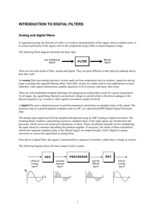
The analog input signal must first be sampled and digitised using an ADC (analog to digital converter). The
resulting binary numbers, representing successive sampled values of the input signal, are transferred to the
processor, which carries out numerical calculations on them. These calculations typically involve multiplying
the input values by constants and adding the products together. If necessary, the results of these calculations,
which now represent sampled values of the filtered signal, are output through a DAC (digital to analog
converter) to convert the signal back to analog form.
Note that in a digital filter, the signal is represented by a sequence of numbers, rather than a voltage or current.
The following diagram shows the basic setup of such a system.
1
2. Advantages of using digital filters
The following list gives some of the main advantages of digital over analog filters.
1. A digital filter is programmable, i.e. its operation is determined by a program stored in the processor's
memory. This means the digital filter can easily be changed without affecting the circuitry (hardware).
An analog filter can only be changed by redesigning the filter circuit.
2. Digital filters are easily designed, tested and implemented on a general-purpose computer or
workstation.
3. The characteristics of analog filter circuits (particularly those containing active components) are
subject to drift and are dependent on temperature. Digital filters do not suffer from these problems,
and so are extremely stable with respect both to time and temperature.
4. Unlike their analog counterparts, digital filters can handle low frequency signals accurately. As the
speed of DSP technology continues to increase, digital filters are being applied to high frequency
signals in the RF (radio frequency) domain, which in the past was the exclusive preserve of analog
technology.
5. Digital filters are very much more versatile in their ability to process signals in a variety of ways; this
includes the ability of some types of digital filter to adapt to changes in the characteristics of the
signal.
6. Fast DSP processors can handle complex combinations of filters in parallel or cascade (series),
making the hardware requirements relatively simple and compact in comparison with the equivalent
analog circuitry.
Operation of digital filters
In this section, we will develop the basic theory of the operation of digital filters. This is essential to an
understanding of how digital filters are designed and used.
Suppose the "raw" signal which is to be digitally filtered is in the form of a voltage waveform described by the
function
V = x(t )
where t is time.
This signal is sampled at time intervals h (the sampling interval). The sampled value at time t = ih is
xi = x (ih)
Thus the digital values transferred from the ADC to the processor can be represented by the sequence
x 0 , x 1 , x 2 , x 3 , ...
corresponding to the values of the signal waveform at
t = 0, h, 2h, 3h, ...
and t = 0 is the instant at which sampling begins.
2
3. At time t = nh (where n is some positive integer), the values available to the processor, stored in memory, are
x 0 , x 1 , x 2 , x 3 , ... x n
Note that the sampled values xn+1, xn+2 etc. are not available, as they haven't happened yet!
The digital output from the processor to the DAC consists of the sequence of values
y 0 , y 1 , y 2 , y 3 , ... y n
In general, the value of yn is calculated from the values x0, x1, x2, x3, ... , xn. The way in which the y's are
calculated from the x's determines the filtering action of the digital filter.
In the next section, we will look at some examples of simple digital filters.
Examples of simple digital filters
The following examples illustrate the essential features of digital filters.
1. Unity gain filter:
y n = xn
Each output value yn is exactly the same as the corresponding input value xn:
y0 = x0
y1 = x1
y 2 = x2
... etc
This is a trivial case in which the filter has no effect on the signal.
2. Simple gain filter:
y n = Kx n
where K = constant.
This simply applies a gain factor K to each input value.
K > 1 makes the filter an amplifier, while 0 < K < 1 makes it an attenuator. K < 0 corresponds to an
inverting amplifier. Example (1) above is simply the special case where K = 1.
3
4. 3. Pure delay filter:
y n = x n-1
The output value at time t = nh is simply the input at time t = (n-1)h, i.e. the signal is delayed by time
h:
y 0 = x -1
y 1 = x0
y 2 = x1
y 3 = x2
... etc
Note that as sampling is assumed to commence at t = 0, the input value x-1 at t = -h is undefined. It is
usual to take this (and any other values of x prior to t = 0) as zero.
4. Two-term difference filter:
y n = x n - x n-1
The output value at t = nh is equal to the difference between the current input xn and the previous
input xn-1:
y 0 = x0 - x -1
y 1 = x1 - x0
y 2 = x2 - x1
y 3 = x3 - x2
... etc
i.e. the output is the change in the input over the most recent sampling interval h. The effect of this
filter is similar to that of an analog differentiator circuit.
4
5. 5. Two-term average filter:
x n + x n-1
yn =
2
The output is the average (arithmetic mean) of the current and previous input:
x 0 + x -1
y0 =
2
x + x0
y1 = 1
2
x 2 + x1
y2 =
2
x3 + x2
y3 =
2
... etc
This is a simple type of low pass filter as it tends to smooth out high-frequency variations in a signal.
(We will look at more effective low pass filter designs later).
6. Three-term average filter:
x n + x n-1 + x n− 2
yn =
3
This is similar to the previous example, with the average being taken of the current and two previous
inputs:
x 0 + x -1 + x -2
y0 =
3
x + x0 + x -1
y1 = 1
3
x + x1 + x0
y2 = 2
3
x3 + x2 + x1
y3 =
3
As before, x-1 and x-2 are taken to be zero.
5
6. 7. Central difference filter:
x n - x n-2
yn =
2
This is similar in its effect to example (4). The output is equal to half the change in the input signal
over the previous two sampling intervals:
x 0 - x -2
y0 =
2
x - x -1
y1 = 1
2
x2 - x0
y2 =
2
x 3 - x1
y3 =
2
... etc
Order of a digital filter
The order of a digital filter is the number of previous inputs (stored in the processor's memory) used to
calculate the current output.
Thus:
1. Examples (1) and (2) above are zero-order filters, as the current output yn depends only on the current input
xn and not on any previous inputs.
2. Examples (3), (4) and (5) are all of first order, as one previous input (xn-1) is required to calculate yn. (Note
that the filter of example (3) is classed as first-order because it uses one previous input, even though the
current input is not used).
3. In examples (6) and (7), two previous inputs (xn-1 and xn-2) are needed, so these are second-order filters.
Filters may be of any order from zero upwards.
Digital filter coefficients
All of the digital filter examples given above can be written in the following general forms:
Zero order: y n = a0xn
First order: y n = a 0 x n + a 1 x n-1
Second order: y n = a 0 x n + a 1 x n-1 + a 2 x n-2
Similar expressions can be developed for filters of any order.
6
7. The constants a0, a1, a2, ... appearing in these expressions are called the filter coefficients. It is the values of
these coefficients that determine the characteristics of a particular filter.
The following table gives the values of the coefficients of each of the filters given as examples above.
Example Order a0 a1 a2
1 0 1 - -
2 0 K - -
3 1 0 1 -
4 1 1 -1 -
1 1
5 1 /2 /2 -
1 1 1
6 2 /3 /3 /3
1
7 2 /2 0 -1/2
SAQ 1 For each of the following filters, state the order of the filter and identify the values of its
coefficients:
(a) y n = 2x n - x n-1
(b) y n = x n-2
(c) y n = x n - 2x n-1 + 2x n-2 + x n-3
Recursive and non-recursive filters
For all the examples of digital filters discussed so far, the current output (yn) is calculated solely from the
current and previous input values (xn, xn-1, xn-2, ...). This type of filter is said to be non-recursive.
A recursive filter is one which in addition to input values also uses previous output values. These, like the
previous input values, are stored in the processor's memory.
The word recursive literally means "running back", and refers to the fact that previously-calculated output
values go back into the calculation of the latest output. The expression for a recursive filter therefore contains
not only terms involving the input values (xn, xn-1, xn-2, ...) but also terms in yn-1, yn-2, ...
From this explanation, it might seem as though recursive filters require more calculations to be performed,
since there are previous output terms in the filter expression as well as input terms. In fact, the reverse is
usually the case: to achieve a given frequency response characteristic using a recursive filter generally requires
a much lower order filter (and therefore fewer terms to be evaluated by the processor) than the equivalent non-
recursive filter. This will be demonstrated later.
7
8. Note
Some people prefer an alternative terminology in which a non-recursive filter is known as
an FIR (or Finite Impulse Response) filter, and a recursive filter as an IIR (or Infinite
Impulse Response) filter.
These terms refer to the differing "impulse responses" of the two types of filter. The
impulse response of a digital filter is the output sequence from the filter when a unit
impulse is applied at its input. (A unit impulse is a very simple input sequence consisting
of a single value of 1 at time t = 0, followed by zeros at all subsequent sampling instants).
An FIR filter is one whose impulse response is of finite duration. An IIR filter is one
whose impulse response theoretically continues for ever because the recursive (previous
output) terms feed back energy into the filter input and keep it going. The term IIR is not
very accurate because the actual impulse responses of nearly all IIR filters reduce virtually
to zero in a finite time. Nevertheless, these two terms are widely used.
Example of a recursive filter
A simple example of a recursive digital filter is given by
y n = x n + y n-1
In other words, this filter determines the current output (yn) by adding the current input (xn) to the previous
output (yn-1):
y 0 = x0 + y -1
y 1 = x1 + y0
y 2 = x2 + y1
y 3 = x3 + y2
... etc
Note that y-1 (like x-1) is undefined, and is usually taken to be zero.
Let us consider the effect of this filter in more detail. If in each of the above expressions we substitute for yn-1
the value given by the previous expression, we get the following:
y0 = x0 + y -1 = x 0
y 1 = x1 + y 0 = x1 + x 0
y 2 = x2 + y 1 = x 2 + x1 + x 0
y 3 = x3 + y 2 = x 3 + x 2 + x1 + x 0
... etc
Thus we can see that yn, the output at t = nh, is equal to the sum of the current input xn and all the previous
inputs. This filter therefore sums or integrates the input values, and so has a similar effect to an analog
integrator circuit.
8
9. This example demonstrates an important and useful feature of recursive filters: the economy with which the
output values are calculated, as compared with the equivalent non-recursive filter. In this example, each output
is determined simply by adding two numbers together. For instance, to calculate the output at time t = 10h, the
recursive filter uses the expression
y 10 = x 10 + y 9
To achieve the same effect with a non-recursive filter (i.e. without using previous output values stored in
memory) would entail using the expression
y 10 = x 10 + x 9 + x 8 + x 7 + x 6 + x 5 + x 4 + x 3 + x 2 + x 1 + x 0
This would necessitate many more addition operations as well as the storage of many more values in memory.
Order of a recursive (IIR) digital filter
The order of a digital filter was defined earlier as the number of previous inputs which have to be stored in
order to generate a given output. This definition is appropriate for non-recursive (FIR) filters, which use only
the current and previous inputs to compute the current output. In the case of recursive filters, the definition can
be extended as follows:
The order of a recursive filter is the largest number of previous input or output values
required to compute the current output.
This definition can be regarded as being quite general: it applies both to FIR and IIR filters.
For example, the recursive filter discussed above, given by the expression
y n = x n + y n-1
is classed as being of first order, because it uses one previous output value (yn-1), even though no previous
inputs are required.
In practice, recursive filters usually require the same number of previous inputs and outputs. Thus, a first-order
recursive filter generally requires one previous input (xn-1) and one previous output (yn-1), while a second-order
recursive filter makes use of two previous inputs (xn-1 and xn-2) and two previous outputs (yn-1 and yn-2); and so
on, for higher orders.
Note that a recursive (IIR) filter must, by definition, be of at least first order; a zero-order recursive filter is an
impossibility. (Why?)
9
10. SAQ 2 State the order of each of the following recursive filters:
(a) y n = 2x n - x n-1 + y n-1
(b) y n = x n-1 - x n-3 - 2y n-1
(c) y n = x n + 2x n-1 + x n-2 - 2y n-1 + y n-2
Coefficients of recursive (IIR) digital filters
From the above discussion, we can see that a recursive filter is basically like a non-recursive filter, with the
addition of extra terms involving previous inputs (yn-1, yn-2 etc.).
A first-order recursive filter can be written in the general form
(a 0 x n + a 1 x n-1 - b 1 y n-1 )
yn =
b0
Note the minus sign in front of the "recursive" term b1yn-1, and the factor (1/b0) applied to all the coefficients.
The reason for expressing the filter in this way is that it allows us to rewrite the expression in the following
symmetrical form:
b 0 y n + b 1 y n-1 = a 0 x n + a 1 x n-1
In the case of a second-order filter, the general form is
a 0 xn + a1 x n −1 + a 2 x n − 2 − b1 y n −1 − b2 y n − 2
yn =
b0
The alternative "symmetrical" form of this expression is
b 0 y n + b 1 y n-1 + b 2 y n-2 = a 0 x n + a 1 x n-1 + a 2 x n-2
Note the convention that the coefficients of the inputs (the x's) are denoted by a's, while the coefficients of the
outputs (the y's) are denoted by b's.
SAQ 3 Identify the values of the filter coefficients for the first-order recursive filter
y n = x n + y n-1
discussed earlier.
Repeat this for each of the filters in SAQ 2.
10
11. The transfer function of a digital filter
In the last section, we used two different ways of expressing the action of a digital filter: a form giving the
output yn directly, and a "symmetrical" form with all the output terms on one side and all the input terms on
the other.
In this section, we introduce what is called the transfer function of a digital filter. This is obtained from the
symmetrical form of the filter expression, and it allows us to describe a filter by means of a convenient,
compact expression. We can also use the transfer function of a filter to work out its frequency response.
First of all, we must introduce the delay operator, denoted by the symbol z-1.
When applied to a sequence of digital values, this operator gives the previous value in the sequence. It
therefore in effect introduces a delay of one sampling interval.
Applying the operator z-1 to an input value (say xn) gives the previous input (xn-1):
z -1 x n = x n-1
Suppose we have an input sequence
x0 = 5
x1 = -2
x2 = 0
x3 = 7
x4 = 10
Then
z -1 x 1 = x 0 = 5
z -1 x 2 = x 1 = - 2
z -1 x 3 = x 2 = 0
and so on. Note that z-1 x0 would be x-1, which is unknown (and usually taken to be zero, as we have already
seen).
Similarly, applying the z-1 operator to an output gives the previous output:
z -1 y n = y n-1
Applying the delay operator z-1 twice produces a delay of two sampling intervals:
z -1 (z -1 x n ) = z -1 x n-1 = x n-2
We adopt the (fairly logical) convention
z -1 z -1 = z -2
11
12. i.e. the operator z-2 represents a delay of two sampling intervals:
z -2 x n = x n-2
This notation can be extended to delays of three or more sampling intervals, the appropriate power of z-1 being
used.
Let us now use this notation in the description of a recursive digital filter. Consider, for example, a general
second-order filter, given in its symmetrical form by the expression
b 0 y n + b 1 y n-1 + b 2 y n-2 = a 0 x n + a 1 x n-1 + a 2 x n-2
We will make use of the following identities:
y n-1 = z -1 y n
y n-2 = z -2 y n
x n-1 = z -1 x n
x n-2 = z -2 x n
Substituting these expressions into the digital filter gives
(b 0 + b 1 z -1 + b 2 z -2 ) y n = (a 0 + a 1 z -1 + a 2 z -2 ) x n
Rearranging this to give a direct relationship between the output and input for the filter, we get
yn a + a 1 z -1 + a 2 z -2
= 0
xn b 0 + b 1 z -1 + b 2 z -2
This is the general form of the transfer function for a second-order recursive (IIR) filter.
For a first-order filter, the terms in z-2 are omitted. For filters of order higher than 2, further terms involving
higher powers of z-1 are added to both the numerator and denominator of the transfer function.
A non-recursive (FIR) filter has a simpler transfer function which does not contain any denominator terms.
The coefficient b0 is usually taken to be equal to 1, and all the other b coefficients are zero. The transfer
function of a second-order FIR filter can therefore be expressed in the general form
yn
= a 0 + a 1 z -1 + a 2 z -2
xn
12
13. For example, the three-term average filter, defined by the expression
x n + x n-1 + x n-2
yn =
3
can be written using the z-1 operator notation as
x n + z -1 x n + z -2 x n (1 + z -1 + z -2 ) x n
yn = =
3 3
The transfer function for the filter is therefore
yn 1 + z -1 + z -2
=
xn 3
The general form of the transfer function for a first-order recursive filter can be written
yn a 0 + a 1 z -1
=
xn b 0 + b 1 z -1
Consider, for example, the simple first-order recursive filter
y n = x n + y n-1
which we discussed earlier. To derive the transfer function for this filter, we rewrite the filter expression using
the z-1 operator:
(1 - z -1 ) y n = x n
Rearranging gives the filter transfer function as
yn 1
=
xn 1 - z -1
As a further example, consider the second-order IIR filter
y n = x n + 2x n-1 + x n-2 - 2y n-1 + y n-2
Collecting output terms on the left and input terms on the right to give the "symmetrical" form of the filter
expression, we get
y n + 2y n-1 - y n-2 = x n + 2x n-1 + x n-2
Expressing this in terms of the z-1 operator gives
(1 + 2z -1 - z -2 ) y n = (1 + 2z -1 + z -2 ) x n
and so the transfer function is
yn 1 + 2z -1 + z -2
=
xn 1 + 2z -1 - z -2
13
14. SAQ 4 Derive the transfer functions of each of the filters in SAQ 2.
Tutorial question
A digital filter is described by the expression
y n = 2x n - x n-1 + 0.8y n-1
(a) State whether the filter is recursive or non-recursive. Justify your answer.
(b) State the order of the filter.
(c) Derive the filter transfer function.
(d) The following sequence of input values is applied to the filter.
x0 = 5
x1 = 16
x2 = 8
x3 = -3
x4 = 0
x5 = 2
Determine the output sequence for the filter, from y0 to y5.
14
15. Answers to Self-Assessment Questions
SAQ 1
a) Order = 1: a0 = 2, a1 = -1
b) Order = 2: a0 = 0, a1 = 0, a2 = 1
c) Order = 3: a0 = 1, a1 = -2, a2 = 2, a3 = 1
SAQ 2
a) Order = 1
b) Order = 3
c) Order = 2
SAQ 3
a0 = 1 a 1 = 0
b0 = 1 b1= -1
For filters listed in SAQ 2:
a) a0 = 2 a1 = -1 b0 = 1 b1 = -1
b) a0 = 0 a1 = 1 a2 = 0 a3 = -1 b0 = 1 b1 = 2 b2 = 0 b3 = 0
c) a0 = 1 a1 = 2 a2 = 1 b0 = 1 b1 = 2 b2 = -1
SAQ 4
yn 2 - z -1
a) =
xn 1 - z -1
yn z -1 - z -3
b) =
xn 1 + 2z -1
yn 1 + 2z -1 + z -2
c) =
xn 1 + 2z -1 - z -2
15