Slides of the Multivariable Control Systems course @ EPFL (2011)

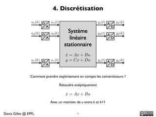
1. 4. Discrétisation
u1 (k) D u1 (t) y1 (t) A y1 (k)
A D
u2 (k) D u2 (t) Système y2 (t) A y2 (k)
A linéaire D
stationnaire
x = Ax + Bu
˙
ur (k) D ur (t) y = Cx + Du yp (t) A yp (k)
A D
Comment prendre explicitement en compte les convertisseurs ?
Résoudre analytiquement
x = Ax + Bu
˙
Avec un maintien de u entre k et k+1
Denis Gillet @ EPFL 1

2. Solution de l’équation d’état
x (t) = Ax (t) + Bu (t)
˙
Solution générale = solution homogène + solution particulière
Cas scalaire Cas vectoriel
x (t0 ) = x0
x (t) = ax (t)
˙ x (t) = Ax (t)
˙
x = eat c2 = ea(t t0 )
x0
1 1
e =1+ + 2
+ 3
+ ...
2! 3!
⇥
1 2 1 3
2 3
x = 1 + a (t t0 ) + a (t t0 ) + a (t t0 ) + . . . x0
2! 3!
2 3
x = a0 + a1 (t t0 ) + a2 (t t0 ) + a3 (t t0 ) + . . .
Par analogie
2 3
x = A0 + A1 (t t0 ) + A2 (t t0 ) + A3 (t t0 ) + . . .
2

3. Solution de l’équation d’état homogène
x (t) = Ax (t)
˙
2 3
x = A0 + A1 (t t0 ) + A2 (t t0 ) + A3 (t t0 ) + . . .
x (t0 ) = A0 x (t0 ) = x0
2
x = A1 + 2A2 (t
˙ t0 ) + 3A3 (t t0 ) + . . .
x (t) = Ax (t)
˙
x (t0 ) = A1
˙
x (t0 ) = Ax (t0 ) = Ax0
˙
x = 2A2 + 6A3 (t
¨ t0 ) + . . .
x (t) = Ax (t)
¨ ˙
x (t0 ) = 2A2
¨
x (t0 ) = Ax (t0 ) = A2 x0
¨ ˙
2 3
⇥
A 2 A 3
x (t) = I + A (t t0 ) + (t t0 ) + (t t0 ) + . . . x0
2! 3!
⇧ ⌅⇤ ⌃
eA(t t0 )
3

4. Exponentielle de matrice
2 3 ⇥
A 2 A 3 Ak k
eA(t t0 )
= I + A (t t0 ) + (t t0 ) + (t t0 ) + . . . = (t t0 )
2! 3! k!
k=0
x (t) = eA(t t0 )
x0
x (t1 ) = eA(t1 t0 )
x (t0 )
x (t2 ) = eA(t2 t1 )
x (t1 ) = eA(t2 t1 ) A(t1 t0 )
e x (t0 )
t 2 = t0
x (t0 ) = eA(t0 t1 ) A(t1 t0 )
e x (t0 )
I = eA(t0 t1 ) A(t1 t0 )
e =M 1
M
⇥ 1
A(t1 t0 )
e = eA(t0 t1 )
=e A(t1 t0 )
4

5. Solution particulière de l’équation d’état
x (t) = Ax (t) + Bu (t)
˙
x (t) = eA(t t0 )
v (t)
AeA(t t0 )
v (t) + eA(t t0 )
v (t) = A eA(t t0 ) v (t) +Bu (t)
˙
⇤ ⇥ ⌅ ⇤ ⇥ ⌅
x(t)
˙ x(t)
⇥ 1
v (t) = eA(t
˙ t0 )
Bu (t) = e A(t t0 )
Bu (t)
t
v (t) = e A( t0 )
Bu ( ) d
t0
t t
x (t) = eA(t t0 )
e A( t0 )
Bu ( ) d = eA(t t0 ) A(t0
e )
Bu ( ) d
t0 t0
t
x (t) = eA(t )
Bu ( ) d
t0
5

6. Solution complète de l’équation d’état
x (t) = Ax (t) + Bu (t)
˙
t
x (t) = e
A(t t0 )
x (t0 ) + A(t
e )
Bu ( ) d
t0
réponse libre + réponse forcée
(produit de convolution)
6

7. Discrétisation
x (t) = Ax (t) + Bu (t)
˙
y (t) = Cx (t) + Du (t)
t
x (t) = eA(t t0 )
x (t0 ) + eA(t )
Bu ( ) d
t0
Convertisseurs AD
kh+h
t0 = kh
x (kh + h) = eAh x (kh) + eA(kh+h )
Bu ( ) d
t = kh + h
kh
t = kh y (kh) = Cx (kh) + Du (kh)
Convertisseurs DA
kh+h
u( ) = u(kh) x (kh + h) = eAh x (kh) + eA(kh+h )
Bu( )d
kh < kh + h ⌅ ⇤⇥ ⇧
kh u(kh)
7

8. Discrétisation
kh+h
x (kh + h) = eAh x (kh) + eA(kh+h )
Bu( )d
⌅ ⇤⇥ ⇧
kh u(kh)
= kh + h ⇥ d = d⇥
⇥
⇧0
x (kh + h) = eAh x (kh) + ⇤ eA Bd ⌅ u (kh)
h
y (kh) = Cx (kh) + Du (kh)
⇤ h ⌅
⌥
⇥
x (k + 1) = eAh
x (k) + ⇧ eA d ⌃ B u (k)
⌦ ↵
⇥ 0
⌦ ↵
y (k) = Cx (k) + Du (k)
8

9. Solution de l’équation d’état analogique,
linéaire et stationnaire + Discrétisation
x (t) = Ax (t) + Bu (t)
˙
y (t) = Cx (t) + Du (t)
t
x (t) = eA(t t0 )
x (t0 ) + eA(t )
Bu ( ) d
t0
x (k + 1) = ⇤⇥ ⌅ x (k) +
⇥ ⇤⇥ ⌅ u (k)
" #
eAh Rh
eA d B
0
y (k) = Cx (k) + Du (k)
9

10. Exponentielle de matrice: Série
A2 2 Ai i
= eAh = I + Ah + h + ... + h + ...
2! i!
⇤ h 2 i
⇥
A 2 A 3 A
= A
e d B = Ih + h + h + ... + hi+1 + . . . B
0 2! 3! (i + 1)!
A A2 2 Ai
=I + h+ h + ... + hi + . . .
2! 3! (i + 1)!
= I + Ah⇥
= ⇥hB
⇥⇥⇥
⇥ I + Ah
= I+
Ah
...
Ah
I+
Ah
2 3 N 1 N
10

11. Discrétisation de systèmes stationnaires
Modèle linéaire Modèle non linéaire
x (t) = f [x (t) , u (t)]
˙
y (t) = g [x (t) , u (t)]
Linéarisation
Contre-
Tangente
réaction
x (t) = Ax (t) + Bu (t)
˙ ˙
x (t)
˜ = A˜ (t) + B u (t)
x ˜
y (t) = Cx (t) + Du (t) y (t)
˜ = C x (t) + D˜ (t)
˜ u
h
Discrétisation exacte =e Ah = eA d B
0
x (k + 1) = ⇥x (k) + u (k) x (k + 1) = ⇥˜ (k) + u (k)
˜ x ˜
y (k) = Cx (k) + Du (k) y (k) = C x (k) + D˜ (k)
˜ ˜ u
11

12. 4.1.8 Double intégrateur: Série
1
u(t) y(t)
s2
y (t) = u(t)
¨
x1 (t) = y(t)
x2 (t) = y(t)
˙
 
x1 (t) = y(t) = x2 (t)
˙ ˙ 0 1 0
x(t) =
˙ x(t) + u(t)
x2 (t) = y (t) = u(t)
˙ ¨ 0 0 1
⇥ ⇤
y(t) = x1 (t) y(t) = 1 0 x(t) + [0] u(t)
12

13. 4.1.8 Double intégrateur: Série
A B
⇧
⇤ ⌥ ⌃
⌅ ⇧ ⌥⌅
⇤ ⌃
0 1 0 ⇥
x=
˙ x+ u et y= 1 0 x
0 0 1 ⌥ ⌃⇧
C
A2 2 Ai i
= eAh = I + Ah + h + ... + h + ...
2! i!
⇥ ⇥ ⇥ 2 ⇥
1 0 0 1 0 0 h 1 h
= + h+ = = eAh
0 1 0 0 0 0 2 0 1
⌅ ⇧ ⇥ ⌃ ⌥
⌦ ⌦ h ⇤ h 2 h ⇥ ⇤
h
1 0 |0 0
= eA d B= d = 2
0
0 1 1 h 1
0 0 0 |0
⌅ 2
⇧⇥ ⇤ ⌅ h2 ⇧
h h 0
= 2 = 2
0 h 1 h
⇤ ⌅ ⇧ 2 ⌃
h ⇥
1 h
x (k + 1) = x (k) + 2 u (k) et y (k) = 1 0 x (k)
0 1 h
13

14. Solution de l’équation d’état
par la transformée de Laplace
x(t) = Ax(t) + Bu(t)
˙
sX(s) x(0) = AX(s) + BU (s)
(sI A)X(s) = x(0) + BU (s)
1 1
X(s) = (sI A) x(0) + (sI A) BU (s)
Rt
x(t) = eAt x(0) + 0
eA(t ⌧)
Bu(⌧ )d⌧
h i
At 1 1
e =L (sI A)
14

15. Algorithme de Leverrier (analogique)
⇥
1
eAt = L 1
(sI A) et = eAh
1 adj (sI A) H0 sn 1 + H1 sn 2 + H2 sn 3 + . . . + Hn 1
(sI A) = =
det (sI A) sn + a1 sn 1 + a2 sn 2 + . . . + an
H0 = I
a1 = tr (AH0 ) H1 = AH0 + a1 I
a2 = 2 tr (AH1 )
1
H2 = AH1 + a2 I
.
. .
.
. .
an 1 = n 1 tr (AHn 2 )
1
Hn 1 = AHn 2 + an 1I
an = n tr (AHn 1 )
1
Hn = AHn 1 + an I = 0
15

16. Double intégrateur: Leverrier
A B
⇧
⇤ ⌥ ⌃
⌅ ⇧ ⌥⌅
⇤ ⌃
0 1 0 ⇥
x=
˙ x+ u et y= 1 0 x
0 0 1 ⌥ ⌃⇧
C
⇥
1
e At
=L 1
(sI A) et = eAh
⇥ ⇥ ⇥
1 0 0 1 0 1
H0 = I = , a1 = tr (AH0 ) = tr = 0, H1 = AH0 + a1 I =
0 1 0 0 0 0
⇥ ⇥
1 1 0 0 0 0
a2 = tr (AH1 ) = tr = 0, H2 = AH1 + a2 I = (contrˆle)
o
2 2 0 0 0 0
⇥ ⇥
1 0 0 1
s+ ⇥
H0 s + H1
1 0 1 0 0 1 s 1
(sI A) = 2 = = 2
s + a1 s + a2 s2 s 0 s
⌅ ⇧ ⇥ ⇤ ⇥ ⇤
1/ 1 2
s s 1 t 1 h
e =L
At 1
= donc e Ah
=
0 1/ 0 1 0 1
s
16

17. Théorème de Cayley-Hamilton
Soit A une matrice n x n:
f (A) = p (A) = 0 An 1
+ 1 An 2
+ ... + n 1I
Les coefficients i sont solution de:
f ( i) = p ( i) i = 1, . . . , n
Les i sont les valeurs propres de A, soit les solutions de:
det ( I A) = | I A| = 0
Pour des valeurs propres de multiplicité mi
f (1) ( i ) = p(1) ( i )
.
.
.
f (mi 1)
( i) = p(mi 1)
( i)
17

18. 4.1.12 Double intégrateur: Cayley-Hamilton
A B
⇧
⇤ ⌥ ⌃
⌅ ⇧ ⌥⌅
⇤ ⌃
0 1 0 ⇥
x=
˙ x+ u et y= 1 0 x
0 0 1 ⌥ ⌃⇧
C
e 1h
= 0 ⇥1 + 1
f (A) = e Ah
= 0A + 1I = 0 ⇥2 +
2h
e 1
⇥ ⇤ ⇥ ⇤ ⇥ ⇤
0 0 1 1
| I A| = = = 2
= 0, = =0
0 0 0 0 1 2
e 1h
= 0 ⇥1 + 1 1= 1
d d
e 2h
= ( 0 ⇥2 + 1) he 2h
= 0 h= 0
d⇥2 d⇥2
⇥ ⇥ ⇥
0 1 1 0 1 h
Ah
e =h +1 =
0 0 0 1 0 1
18

19. 4.2 Solution de l’équation d’état discrète linéaire
x (k + 1) = ⇥x (k) + u (k)
y (k) = Cx (k) + Du (k)
x(k0 + 1) = ⇥x(k0 ) + u(k0 )
x(k0 + 2) = ⇥x(k0 + 1) + u(k0 + 1)
x(k0 + 2) = ⇥ [⇥x(k0 ) + u(k0 )] + u(k0 + 1)
x(k0 + 2) = ⇥2 x(k0 ) + ⇥ u(k0 ) + u(k0 + 1)
x(k0 + 3) = ⇥x(k0 + 2) + u(k0 + 2) ⇥
x(k0 + 3) = ⇥ ⇥ x(k0 ) + ⇥ u(k0 ) + u(k0 + 1) + u(k0 + 2)
2
x(k0 + 3) = ⇥3 x(k0 ) + ⇥2 u(k0 ) + ⇥ u(k0 + 1) + u(k0 + 2)
k 1
x(k) = ⇥k k0
x(k0 ) + ⇥k i 1
u(i)
i=k0
réponse libre + réponse forcée
(produit de convolution)
19

20. Matrice de transfert discrète
x (k + 1) = ⇥x (k) + u (k) CI nulles
y (k) = Cx (k) + Du (k)
zX(z) ⇥X(z) = U (z)
Y (z) = CX(z) + DU (z)
(zI ⇥)X(z) = U (z)
Y (z) = CX(z) + DU (z)
X(z) = (zI ⇥) 1 U (z) ⇥
Y (z) = C (zI ⇥) 1 U (z)⇥ + DU (z)
Y (z) = C(zI ⇥) 1 + D U (z) ⇥ H(z)U (z)
u(k) y(k) U (z) Y (z)
Modèle d’état H(z)
linéaire discret
x(k)
20

21. Matrice de transfert discrète
h i
1
H(z) = C(zI ) +D Y (z) = H(z)U (z)
2 3 2 32 3
Y1 (z) H11 (z) H12 (z) ··· H1r (z) U1 (z)
6 Y2 (z) 7 6 H21 (z) H22 (z) H2r (z) 76 U2 (z) 7
6 7 6 76 7
6 .
. 7=6 .
. .. .
. 76 .
. 7
4 . 5 4 . . . 54 . 5
Yp (z) Hp1 (z) Hp2 (z) ··· Hpr (z) Ur (z)
0 .
.
. .
.
Uj (z) Hij (z) .
.
.
. . Yi (z)
0 .
.
21

22. Algorithme de Leverrier (discret)
1
H (z) = C (zI ⇥) +D
1 adj (zI ) H0 z n 1 + H 1 z n 2 + H2 z n 3 + . . . + Hn 1
(zI ) = =
det (zI ) z n + a1 z n 1 + a2 z n 2 + . . . + an
H0 = I
a1 = tr ( H0 ) H1 = H0 + a1 I
a2 = 2 tr (
1
H1 ) H2 = H1 + a2 I
.
. .
.
. .
an 1 = n 1 tr ( Hn 2 )
1
Hn 1 = Hn 2 + an 1I
an = n tr ( Hn 1 )
1
Hn = Hn 1 + an I = 0
22

23. 4.2.4 Double intégrateur: Matrice de transfert
⇥
1 h
= H (z) = C (zI ⇥)
1
+D
0 1
⇥
1 adj (zI ) Iz + H1 1 z 1 h
(zI ) = = 2 = 2
det (zI ) z + a1 z + a2 z 2z + 1 0 z 1
a1 = tr ( ) = 2
⇥ ⇤ ⇥ ⇤ ⇥ ⇤
1 h 1 0 1 h
H1 = + a1 I = 2 =
0 1 0 1 0 1
⇥ ⇤
1 0
a2 = 2 tr (
1
H1 ) = 1
2 tr =1
0 1
⇥ ⇤ ⇥ ⇤ ⇥ ⇤
1 0 1 0 0 0
H2 = H1 + a2 I = + = cqfd
0 1 0 1 0 0
⌅ ⇧⌅ ⇤ ⇧
⇥ z 1 h h2 2 1
H (z) = 1 0 2
0 z 1 h (z 1)
⌅ ⇤ ⇧ ⇤
⇥ h2 2 1 (z 1) h 2 + h2
2
h2 z + 1
H (z) = z 1 h 2 = =
h (z 1) (z
2
1) 2 (z 1)2

24. Stabilité
1
H (z) = C (zI ⇥) +D
Cadj(zI ⇥) H (z)
H(z) = +D =
det(zI ⇥) det(zI ⇥)
⇤ ⌅
H11 (z) ... H1r (z) ⇥
⌥ . . Hij (z)
H (z) = ⇧ .
. .
. ⌃ = [Hij (z)] =
det (zI )
Hp1 (z) ··· Hpr (z)
Pˆles zi des Hij solution de: det (zI
o )=0
Valeurs propres vi de solution de: det ( I )=0
zi = vi
Asymptotiquement stable si: |vi | < 1 pour i = 1, . . . , n
24

25. 4.1.13 Exemple: Entraînement discret
⇤ ⌅ ⇤ ⌅
u (k) u (t) x =
˙
0 1
x+
0
u y (t) y (k) x (k + 1) = ⇥x (k) + u (k)
D 0 a b A
A ⇥ D y (k) = Cx (k)
y = 1 0 x
" # " #
1 1
a eah 1 b
1
a eah 1 h
⇥=e Ah
= = exemple: 4.1.13
0 e ah a eah
1
⇤ ⇥ ⇥ ⌅
1 Iz + H1 1 z eah 1
a eah 1
(zI ) = 2 =
z + a1 z + a2 (z eah ) (z 1) 0 z 1
1
H (z) = C (zI ⇥) +D Inutile ! Les valeurs propres donnent la mˆme info
e
⇤ ⇥ ⌅ ⇧
1 1
a e ah
1 ⇥ 1 = z1 = 1
| I |= =( 1) ah
e =0⇥ = z2 = eah
0 eah 2
25

26. Systèmes discrets linéaires et stationnaires
Solution k 1
x (k + 1) = ⇥x (k) + u (k) x (k) = ⇥k k0 x (k0 ) + ⇥k l 1
u (l)
⌅ ⇤⇥ ⇧
y (k) = Cx (k) + Du (k) l=k0
R´ponse libre
e ⌅ ⇤⇥ ⇧
R´ponse forc´e
e e
Matrice de transfert et stabilité
⇥
1
Y (z) = C (zI ⇥) + D U (z) = H (z) U (z)
⇤ ⌅
H11 (z) ... H1r (z) ⇥
⌥ . . Hij (z)
H (z) = ⇧ .
. .
. ⌃ = [Hij (z)] =
det (zI )
Hp1 (z) ··· Hpr (z)
Pˆles zi des Hij solution de: det (zI
o )=0
Valeurs propres vi de solution de: det ( I )=0
zi = vi
Asymptotiquement stable si: |vi | < 1 pour i = 1, . . . , n
26