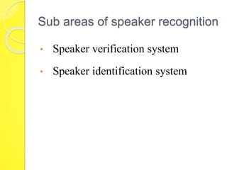
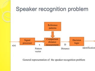
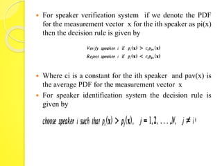
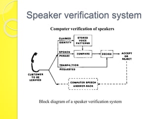
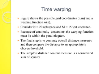
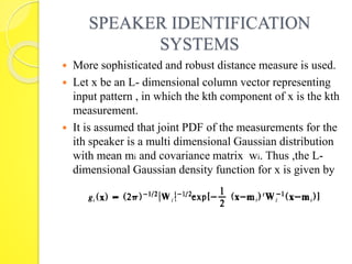
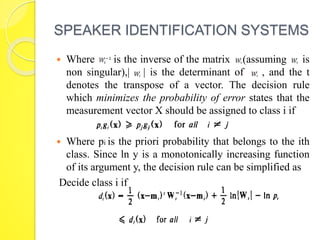
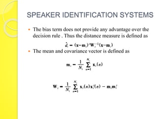
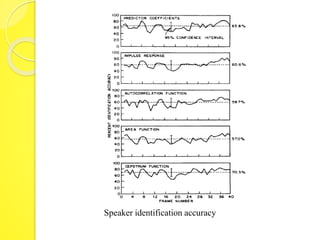
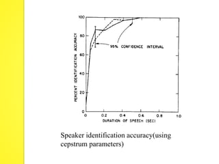
SPEAKER RECOGNITION 
SYSTEMS 
BY 
NAMRATHA D’CRUZ
Sub areas of speaker recognition 
• Speaker verification system 
• Speaker identification system
Speaker recognition problem 
Signal 
processor 
Comparison 
distance 
measurement 
Decision 
logic 
Reference 
patterns 
s(n) x D 
Pattern Distance identification 
vector 
General representation of the speaker recognition problem
 A representation of the speech signal is obtained 
using digital speech processing techniques 
 which preserve the features of the speech signal 
that are relevant to speaker identity. 
 The resulting pattern is compared to previously 
prepared reference patterns. 
 Decision logic is used to make a choice among 
available alternatives
 For speaker verification system if we denote the PDF 
for the measurement vector x for the ith speaker as pi(x) 
then the decision rule is given by 
 Where ci is a constant for the ith speaker and pav(x) is 
the average PDF for the measurement vector x 
 For speaker identification system the decision rule is 
given by
Speaker verification system 
Computer verification of speakers 
Block diagram of a speaker verification system
 Online digital speaker verification system was 
developed by Rosenberg and others. 
 The person wishing to be verified first enters his 
claimed identity. 
 On request from verification system utters his 
verification phrase, and requests some transaction to 
be made in the event he is verified. 
 The spoken utterance is processed to obtain a 
pattern which is compared to the stored reference 
patterns for the claimed identity.
 On the basis of the transaction requested the error mix 
constant (Ci) is determined . 
 Based on error mix constant decision to accept or reject 
is made.
Accept 
Reject 
Signal processing aspects of the speaker verification system
Signal Processing Parts Of The Speaker 
Verification System 
End point detection system: the sample 
utterances which occurs somewhere within a pre 
selected time interval is located. 
Pitch detector : it is used to measure the pitch 
contour of the utterance. 
Energy measurements: short-time energy 
measurements is made to give energy contours.
Signal Processing Parts Of The Speaker 
Verification System 
LPC analysis: is used to give predictor parameter 
contours. 
 LPC is a tool used for representing the spectral 
envelope of a digital signal of speech 
in compressed form, using the information of a linear 
predictive model. 
 Autocorrelation formulation method is used. 
Formant analysis: estimates of the formant 
locations is made. 
LPF: 16hz low pass is used
Measurement contours for the test utterance “we 
were away a year ago” 
 Data are estimated at 100 times per second 
 Smoothened by 16hz LPF, linear phase, FIR 
digital filter.
Pitch period and intensity contours of an utterance used in speaker 
verification
Plot of first 3 formants ,pitch and intensity for a speaker 
verification utterance
Plots of the first 8 LPC coefficients for a speaker verification 
utterance
 After the desired parametric representation has been 
computed it is compared with the corresponding 
reference patterns for the speaker whose identity is 
claimed. 
 Speaker is generally not able to speak at precisely the 
same rate for different repetitions of the verification 
phase. 
 As a solution to this problem non linear time warping of 
the input patterns is done to obtain the best possible 
registration between stored pattern and the measured 
patterns for speakers sample utterance.
Time warping 
 The time scale t of a reference utterance is warped so 
that significant events in some measurement contour a(t) 
line up with the same significant events in the reference 
contour r(t). 
 The warping function is assumed to be 
τ=α t+q(t) 
Where 
q(t) - is the non linear time warp function 
α – average slope of the time warp function
Time warping 
 Boundary condition s are imposed to ensure that the 
beginning and ending points of both the sample and 
reference utterances line up properly. 
 The boundary conditions are: 
τ1=α t1+q(t1) 
τ2=α t2+q(t2) 
 Function q(t) and constant α have to be chosen so as to 
best align the measured contours. 
 Simpler and faster solution is to utilize the method of 
dynamic programming to optimally choose a constrained 
warping function.
Illustration of time warping
Time warping 
 Consider time warping for a pair of contours which are 
sampled at a discrete set of points . 
 Let the points be in the measured contour be labeled 
n=1,2,…,N. 
 Let the points in the reference contour be labeled 
m=1,2,…,M. 
 Time warping function w is chosen as 
m=w(n)
Time warping 
 The boundary on w(n) conditions are: 
w(1) = 1 beginning points 
w(N) = M ending points 
 To limit the degree of non linearity of the warping 
function mild continuity condition is imposed 
 That the warping function w cannot change by more 
than 2 grid points at any index n 
w(n+1)-w(n) = 0,1,2 if w(n) != w(n-1) 
= 1,2 if w(n) = w(n-1) 
 Thus slope of warping function is either 0,1 or 2
Time warping 
 To determine which of the conditions of equation to use 
at grid index n requires the use of similarity measure 
between the reference data measured at grid index n and 
the test data measured at grid index m. 
 The similarity measure is used to determine the path of 
the warping function which minimizes the max total 
distance ,subject to constraints of continuity equation.
An example of a typical time warping
Time warping 
 Figure shows the possible grid coordinates (n,m) and a 
warping function w(n). 
 Consider N = 20 reference and M = 15 test utterance. 
 Because of continuity constraints the warping function 
must lie within the parallelogram. 
 The final step is to compute overall distance measures 
and then compare the distance to an appropriately 
chosen threshold. 
 The simplest distance contour measure is a normalized 
sum of squares .
Distance measure 
 For the jth measurement contour ,the distance dj would 
be of the form 
 Where ajs (i) is the value of the jth measurement contour 
at time i 
 ajr (i) ) is the value of the jth reference contour at time 
i, and σaj(i) is the standard deviation of the jth 
measurement at time i
Distance measure 
 The distance function is given by 
 Where wj is the jth weight chosen on the basis of the 
effectiveness of the jth measurement in verifying the 
speaker.
SPEAKER IDENTIFICATION 
SYSTEMS 
 Almost similar to the speaker verification systems 
 Main difference is choice of parameters to make 
distance measurements. 
 N distance measurements have to be made rather than 1. 
 Final decision is to choose the speaker whose reference 
patterns are closest in distance to the sample patterns.
SPEAKER IDENTIFICATION 
SYSTEMS 
 More sophisticated and robust distance measure is used. 
 Let x be an L- dimensional column vector representing 
input pattern , in which the kth component of x is the kth 
measurement. 
 It is assumed that joint PDF of the measurements for the 
ith speaker is a multi dimensional Gaussian distribution 
with mean mi and covariance matrix wi. Thus ,the L-dimensional 
Gaussian density function for x is given by
SPEAKER IDENTIFICATION SYSTEMS 
 Where is the inverse of the matrix (assuming is 
non singular),| | is the determinant of , and the t 
denotes the transpose of a vector. The decision rule 
which minimizes the probability of error states that the 
measurement vector X should be assigned to class i if 
 Where pi is the priori probability that belongs to the ith 
class. Since ln y is a monotonically increasing function 
of its argument y, the decision rule can be simplified as 
Decide class i if
SPEAKER IDENTIFICATION SYSTEMS 
 The bias term does not provide any advantage over the 
decision rule . Thus the distance measure is defined as 
 The mean and covariance vector is defined as
Examples of some measured parameters
Speaker identification accuracy
Speaker identification accuracy(using 
cepstrum parameters)
Speaker recognition systems

Speaker recognition systems

  • 1.
    SPEAKER RECOGNITION SYSTEMS BY NAMRATHA D’CRUZ
  • 2.
    Sub areas ofspeaker recognition • Speaker verification system • Speaker identification system
  • 3.
    Speaker recognition problem Signal processor Comparison distance measurement Decision logic Reference patterns s(n) x D Pattern Distance identification vector General representation of the speaker recognition problem
  • 4.
     A representationof the speech signal is obtained using digital speech processing techniques  which preserve the features of the speech signal that are relevant to speaker identity.  The resulting pattern is compared to previously prepared reference patterns.  Decision logic is used to make a choice among available alternatives
  • 5.
     For speakerverification system if we denote the PDF for the measurement vector x for the ith speaker as pi(x) then the decision rule is given by  Where ci is a constant for the ith speaker and pav(x) is the average PDF for the measurement vector x  For speaker identification system the decision rule is given by
  • 6.
    Speaker verification system Computer verification of speakers Block diagram of a speaker verification system
  • 7.
     Online digitalspeaker verification system was developed by Rosenberg and others.  The person wishing to be verified first enters his claimed identity.  On request from verification system utters his verification phrase, and requests some transaction to be made in the event he is verified.  The spoken utterance is processed to obtain a pattern which is compared to the stored reference patterns for the claimed identity.
  • 8.
     On thebasis of the transaction requested the error mix constant (Ci) is determined .  Based on error mix constant decision to accept or reject is made.
  • 9.
    Accept Reject Signalprocessing aspects of the speaker verification system
  • 10.
    Signal Processing PartsOf The Speaker Verification System End point detection system: the sample utterances which occurs somewhere within a pre selected time interval is located. Pitch detector : it is used to measure the pitch contour of the utterance. Energy measurements: short-time energy measurements is made to give energy contours.
  • 11.
    Signal Processing PartsOf The Speaker Verification System LPC analysis: is used to give predictor parameter contours.  LPC is a tool used for representing the spectral envelope of a digital signal of speech in compressed form, using the information of a linear predictive model.  Autocorrelation formulation method is used. Formant analysis: estimates of the formant locations is made. LPF: 16hz low pass is used
  • 12.
    Measurement contours forthe test utterance “we were away a year ago”  Data are estimated at 100 times per second  Smoothened by 16hz LPF, linear phase, FIR digital filter.
  • 13.
    Pitch period andintensity contours of an utterance used in speaker verification
  • 14.
    Plot of first3 formants ,pitch and intensity for a speaker verification utterance
  • 15.
    Plots of thefirst 8 LPC coefficients for a speaker verification utterance
  • 16.
     After thedesired parametric representation has been computed it is compared with the corresponding reference patterns for the speaker whose identity is claimed.  Speaker is generally not able to speak at precisely the same rate for different repetitions of the verification phase.  As a solution to this problem non linear time warping of the input patterns is done to obtain the best possible registration between stored pattern and the measured patterns for speakers sample utterance.
  • 17.
    Time warping The time scale t of a reference utterance is warped so that significant events in some measurement contour a(t) line up with the same significant events in the reference contour r(t).  The warping function is assumed to be τ=α t+q(t) Where q(t) - is the non linear time warp function α – average slope of the time warp function
  • 18.
    Time warping Boundary condition s are imposed to ensure that the beginning and ending points of both the sample and reference utterances line up properly.  The boundary conditions are: τ1=α t1+q(t1) τ2=α t2+q(t2)  Function q(t) and constant α have to be chosen so as to best align the measured contours.  Simpler and faster solution is to utilize the method of dynamic programming to optimally choose a constrained warping function.
  • 19.
  • 20.
    Time warping Consider time warping for a pair of contours which are sampled at a discrete set of points .  Let the points be in the measured contour be labeled n=1,2,…,N.  Let the points in the reference contour be labeled m=1,2,…,M.  Time warping function w is chosen as m=w(n)
  • 21.
    Time warping The boundary on w(n) conditions are: w(1) = 1 beginning points w(N) = M ending points  To limit the degree of non linearity of the warping function mild continuity condition is imposed  That the warping function w cannot change by more than 2 grid points at any index n w(n+1)-w(n) = 0,1,2 if w(n) != w(n-1) = 1,2 if w(n) = w(n-1)  Thus slope of warping function is either 0,1 or 2
  • 22.
    Time warping To determine which of the conditions of equation to use at grid index n requires the use of similarity measure between the reference data measured at grid index n and the test data measured at grid index m.  The similarity measure is used to determine the path of the warping function which minimizes the max total distance ,subject to constraints of continuity equation.
  • 23.
    An example ofa typical time warping
  • 24.
    Time warping Figure shows the possible grid coordinates (n,m) and a warping function w(n).  Consider N = 20 reference and M = 15 test utterance.  Because of continuity constraints the warping function must lie within the parallelogram.  The final step is to compute overall distance measures and then compare the distance to an appropriately chosen threshold.  The simplest distance contour measure is a normalized sum of squares .
  • 25.
    Distance measure For the jth measurement contour ,the distance dj would be of the form  Where ajs (i) is the value of the jth measurement contour at time i  ajr (i) ) is the value of the jth reference contour at time i, and σaj(i) is the standard deviation of the jth measurement at time i
  • 26.
    Distance measure The distance function is given by  Where wj is the jth weight chosen on the basis of the effectiveness of the jth measurement in verifying the speaker.
  • 27.
    SPEAKER IDENTIFICATION SYSTEMS  Almost similar to the speaker verification systems  Main difference is choice of parameters to make distance measurements.  N distance measurements have to be made rather than 1.  Final decision is to choose the speaker whose reference patterns are closest in distance to the sample patterns.
  • 28.
    SPEAKER IDENTIFICATION SYSTEMS  More sophisticated and robust distance measure is used.  Let x be an L- dimensional column vector representing input pattern , in which the kth component of x is the kth measurement.  It is assumed that joint PDF of the measurements for the ith speaker is a multi dimensional Gaussian distribution with mean mi and covariance matrix wi. Thus ,the L-dimensional Gaussian density function for x is given by
  • 29.
    SPEAKER IDENTIFICATION SYSTEMS  Where is the inverse of the matrix (assuming is non singular),| | is the determinant of , and the t denotes the transpose of a vector. The decision rule which minimizes the probability of error states that the measurement vector X should be assigned to class i if  Where pi is the priori probability that belongs to the ith class. Since ln y is a monotonically increasing function of its argument y, the decision rule can be simplified as Decide class i if
  • 30.
    SPEAKER IDENTIFICATION SYSTEMS  The bias term does not provide any advantage over the decision rule . Thus the distance measure is defined as  The mean and covariance vector is defined as
  • 31.
    Examples of somemeasured parameters
  • 32.
  • 33.