Downloaded 66 times

![BRIEF HISTORY
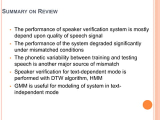
Research in the field of speaker recognition was initially
carried out in 1950s in Bell laboratories using isolated digits
[1].
1960- 1990 most of the research was focused on extraction of
speaker specific information from the speech data, and
development of text dependent speaker verification system.
In 1990-2005 the speaker recognition method shifted from
template based pattern matching to statistical modeling.
Different statistical modeling method like GMM and GMM-
UBM are proposed.
2005- 2014 most of the research was focused on
compensation of mismatches and development of practical
authentication systems. Different compensation methods like
JAFA, i-vectors and LDA, WCCN, PLDA are proposed.
1. K. H. Davis, et. al., “Automatic recognition of spoken
digits,” J.A.S.A., 24 (6), pp. 637-642, 1952.](https://image.slidesharecdn.com/presentationthesis-150624180201-lva1-app6892/85/SPEAKER-VERIFICATION-4-320.jpg)
![PREPROCESSING
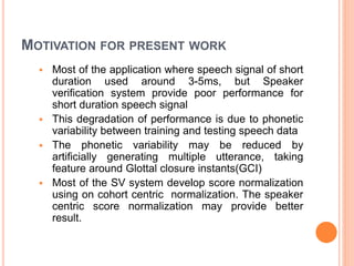
Preprocessing is an important step in a speaker verification
system. This also called voice activity detection (VAD).
VAD separates speech region from non-speech regions[2-3]
It is very difficult to implement a VAD algorithm which works
consistently for different type of data
VAD algorithms can be classified in two groups
Feature based approach
Statistical model based approach
Each of the VAD method have its own merits and demerits
depending on accuracy, complexity etc.
Due to simplicity most of the speaker verification systems use
signal energy for VAD.
2. J. P. Campbell, “Speaker Recognition: A Tutorial,” Proc. IEEE, vol. 85,
no. 9, pp. 1437–1462, September 1997.
3. D. A. Reynolds and R. C. Rose, “Robust text-independent speaker
identification using Gaussian mixture speaker models,” IEEE Trans. on
speech and audio processing, vol. 3, no. 1, pp. 72–83, January 1995.](https://image.slidesharecdn.com/presentationthesis-150624180201-lva1-app6892/85/SPEAKER-VERIFICATION-6-320.jpg)
![FEATURE EXTRACTION
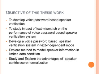
The speech signal along with speaker information contains
many other redundant information like recording sensor,
channel, environment etc.
The speaker specific information in the speech signal[2]
Unique speech production system
Physiological
Behavioral aspects
Feature extraction module transforms speech to a set of
feature vectors of reduce dimensions
To enhance speaker specific information
Suppress redundant information[2-4]
4. F. Bimbot, J. Bonastreand, C. Fredouille, G. Gravier, I. Chagnolleau, S.
Meignier, T. Merlin, J. Garcia, D. Delacretaz, and D. A. Reynolds, “A
tutorial on text-independent speaker verification,” EURASIP Journal on
Applied Signal Processing, vol. 4, pp. 430–451, 2004.](https://image.slidesharecdn.com/presentationthesis-150624180201-lva1-app6892/85/SPEAKER-VERIFICATION-7-320.jpg)
![SPEAKER MODELING
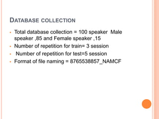
Speaker models the statistical information present in the
feature vectors it enhances the speaker information and
suppress the redundant information
For text independent speaker verification speaker
modeling technique used is vector quantization(VQ),
Gaussian mixer model(GMM)[5], GMM-universal back
ground model(GMM-UBM)[6], Artificial neural
network(ANN)and support vector machine(SVM)
The Gaussian mixer model is most widely used for
speaker verification systems
5. D. A. Reynolds, “Speaker identification and verification using
Gaussian mixture speaker models,” Speech Communication, vol.
17, pp. 91–108, March 1995.
6. D. A. Reynolds, T. F. Quatieri, and R. B. Dunn, “Speaker
verification using adapted Gaussian mixture models,” Digital Signal
Processing, vol. 10, pp. 19–41, January 2000.](https://image.slidesharecdn.com/presentationthesis-150624180201-lva1-app6892/85/SPEAKER-VERIFICATION-11-320.jpg)
![Pattern comparison
Testing phase test feature vectors are compared
with claimed model to get similarity between
training and testing speech
Different similarity measure is done for used
modeling method
Euclidean distance [8] for VQ , log likelihood
score(LLS)[7] and log likelihood score ratio(LLSR)
for GMM-UBM.
7. D. A. Reynolds and R. C. Rose, “Robust text-independent speaker
identification using Gaussian mixture speaker models,” IEEE Trans. on
speech and audio processing, vol. 3, no. 1, pp. 72–83, January 1995
8. F. K. Soong and A. E. Rosenberg, “On the use of instantaneous and
transitional spectral information in speaker recognition,” IEEE Trans.
Acoustics, Speech and Signal Processing, vol. 36, no. 6, pp. 871–879, June
1988](https://image.slidesharecdn.com/presentationthesis-150624180201-lva1-app6892/85/SPEAKER-VERIFICATION-13-320.jpg)
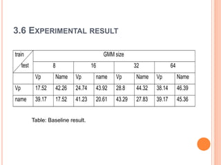
![PERFORMANCE MEASURE:
A perfect SV system should accept all true claim and reject
all the false claims
Depending on the variability between the training and
testing speech some true claim may be rejected and some
false claim may be accepted
Therefore the speaker verification performance is
measured in term of false rejection rate (FRR) and false
acceptance rate (FAR), more meaningfully in term of equal
error rate(EER)[9].
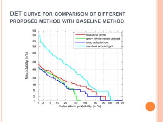
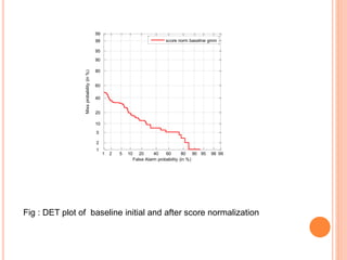
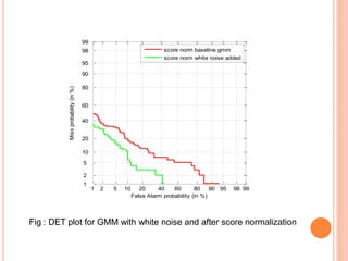
In order to improve the visualization of the SV
performance, the detection error tradeoff(DTF) curve is
used to performance measure
9.F. Bimbot, J. Bonastreand, C. Fredouille, G. Gravier, I. Chagnolleau, S.
Meignier, T. Merlin, J. Garcia, D. Delacretaz, and D. A. Reynolds, “A tutorial
on text-independent speaker verification,” EURASIP Journal on Applied
Signal Processing, vol. 4, pp. 430–451, 2004](https://image.slidesharecdn.com/presentationthesis-150624180201-lva1-app6892/85/SPEAKER-VERIFICATION-14-320.jpg)
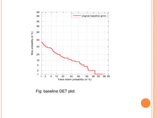
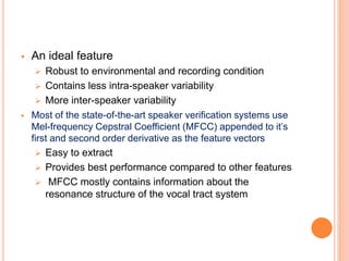
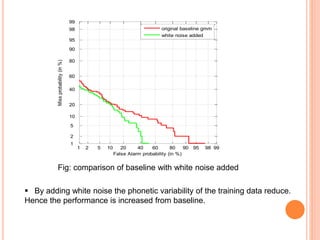
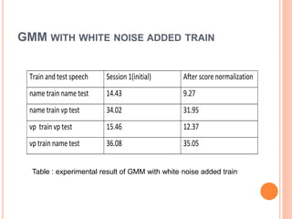
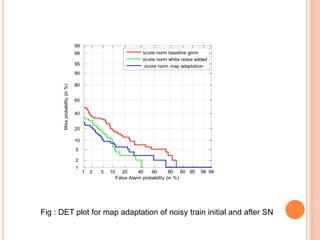
![GENERATION OF MULTIPLE UTTERANCE BY ADDING
WHITE NOISE TO TRAINING SPEECH
Motivation
It covers entire spectrum of speech signal
Addition of white noise will reduce phonetic variability as
it covers entire spectrum
Feature are calculated white noise added for
training and clear for testing
Modeling of train with white noise added, and test
data is clear
White noise used range [-10,-5,0,+5,+10,+20]db
VAD used in clean speech for reference index
Reference index is used to find speech region](https://image.slidesharecdn.com/presentationthesis-150624180201-lva1-app6892/85/SPEAKER-VERIFICATION-22-320.jpg)
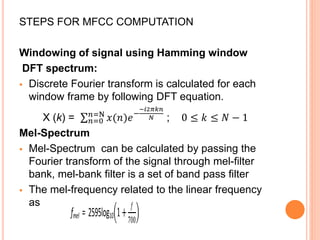
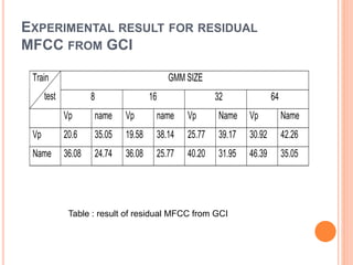
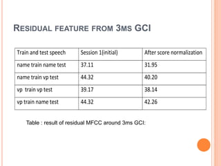
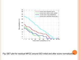
![RESIDUAL MFCC FROM GCI
Computation of residual phase through Linear
prediction analysis
The speech signal produced is convolution of
excitation source and vocal track system
The speaker verification system required speaker
specific information
The feature around glottal closure instants (GCI)
are more speaker specific[10]
10. B. Yanganarayana and P. Satyanarayana Murty, “Enhancement of
reverberant speech using LP residual signal,”IEEE Trans.Speech Audio
Process.,vol. 14, pp. 774-784, May 2006.](https://image.slidesharecdn.com/presentationthesis-150624180201-lva1-app6892/85/SPEAKER-VERIFICATION-28-320.jpg)
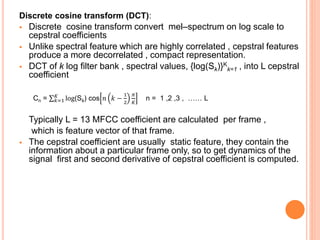
![ZERO FREQUENCY FILTERING (ZFF) METHOD
The ZFF method is most useful for evaluating the
various parameter of prosodic parameter
It is the best available method to calculate
expressive parameter for various emotions
The feature around CGI can be computed using
ZFF[11]
Periodically located epoch in voiced speech signal
represent the glottal closure instants
11. K. S. R. Murty and B. Yegnanarayana, “Epoch extraction from speech
signals,” IEEE Trans. Audio, Speech and Language Process., vol. 16, no.
8, pp. 1602–1614, Nov. 2008](https://image.slidesharecdn.com/presentationthesis-150624180201-lva1-app6892/85/SPEAKER-VERIFICATION-29-320.jpg)
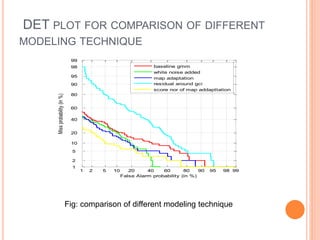

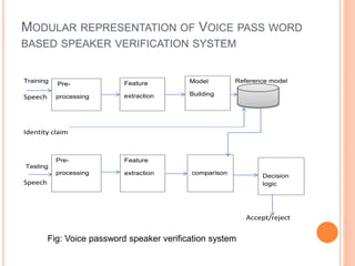
This document outlines a proposed study on developing a voice password-based speaker verification system. It will explore methods for modeling speakers with limited data, such as artificially generating multiple utterances from short speech segments. The study aims to reduce phonetic variability between training and test data. It will also examine score normalization techniques, comparing cohort-centric normalization typically used to a proposed speaker-centric approach. The goal is to build a text-independent voice password system that can reliably verify identities from short speech samples, improving security and enabling remote access applications.


![Getting Started with Apache Spark: Big Data Made Simple [Free Meetup]](https://cdn.slidesharecdn.com/ss_thumbnails/apachesparkgettingstarted-260203175547-8361bcc3-thumbnail.jpg?width=640&height=640&fit=bounds)


