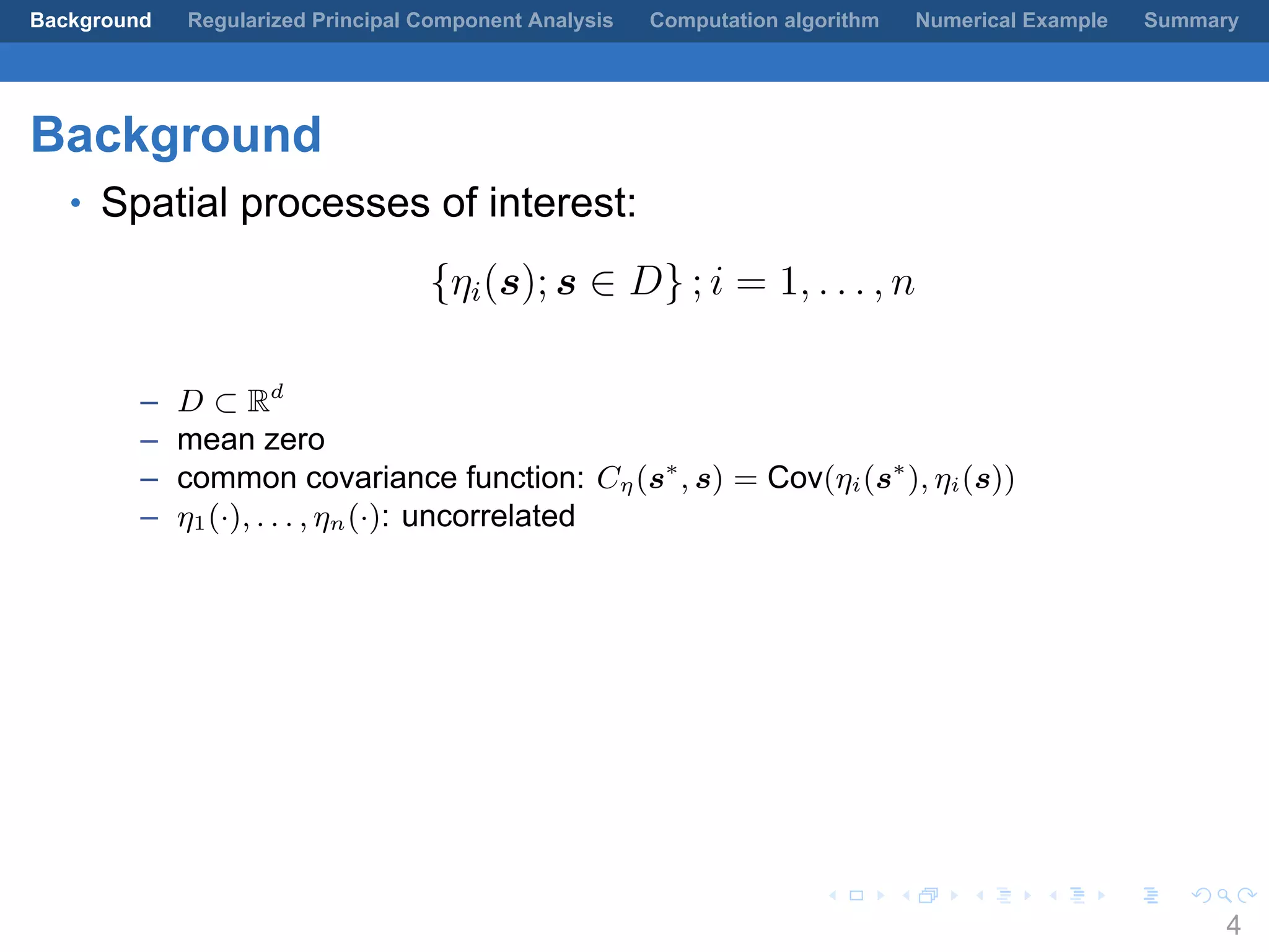
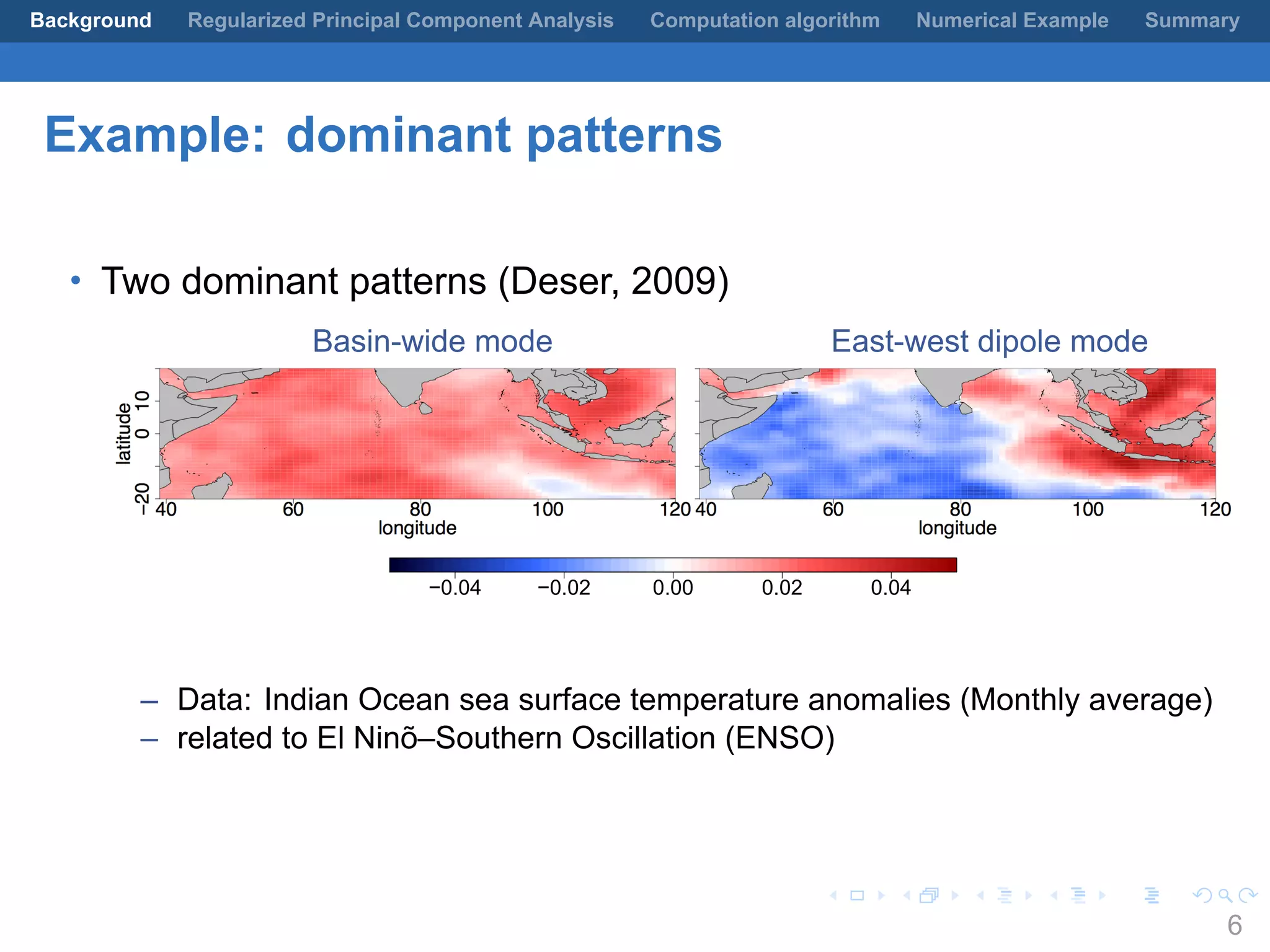
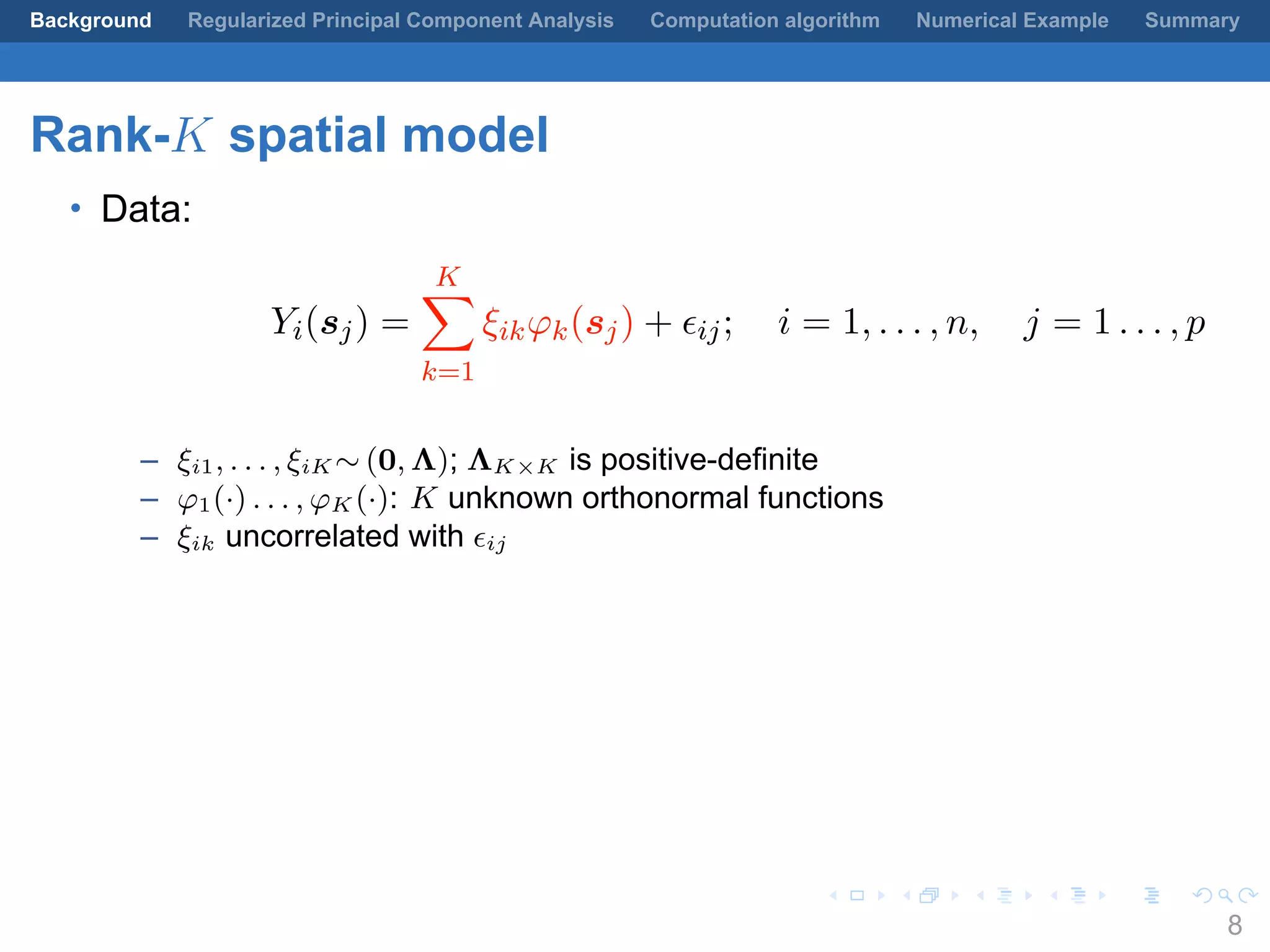
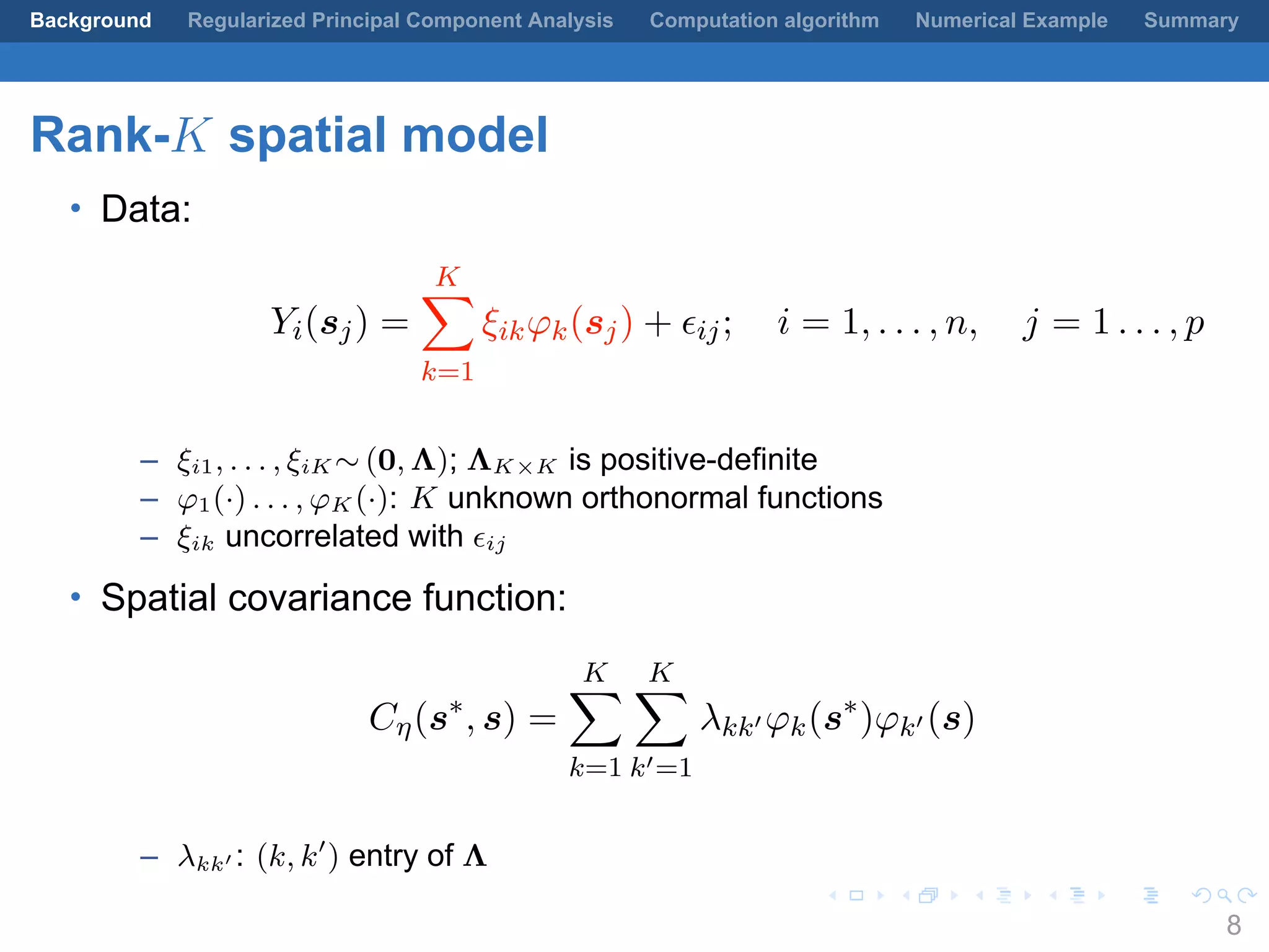
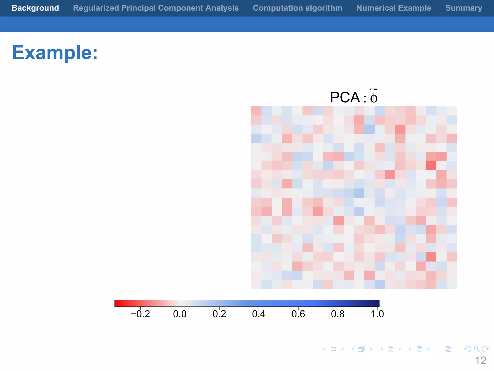
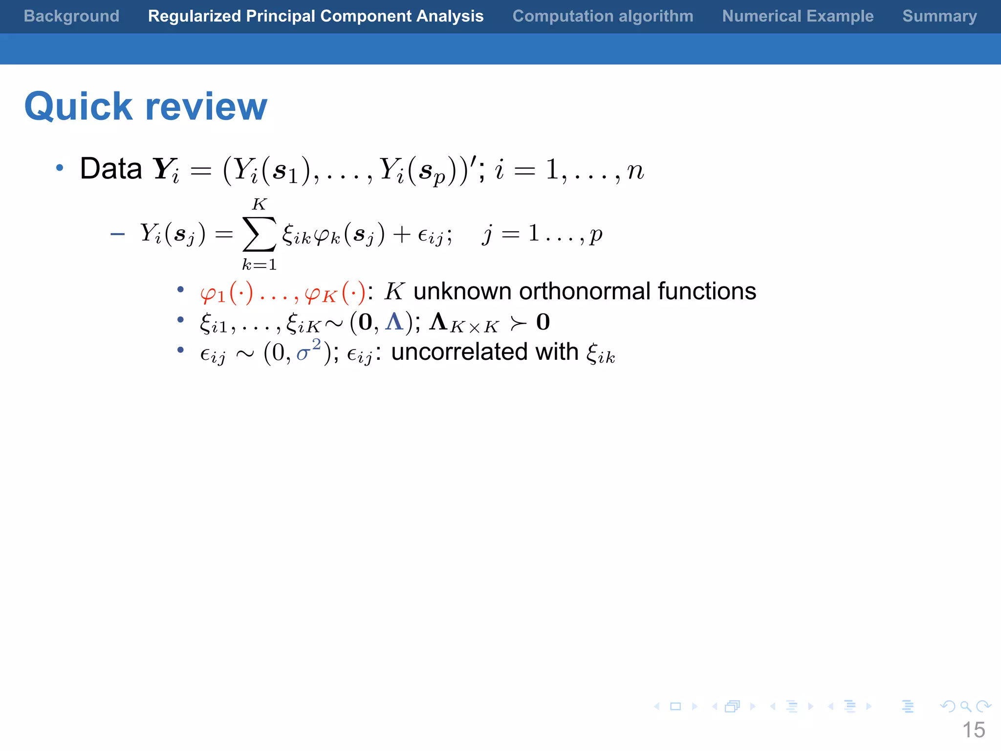
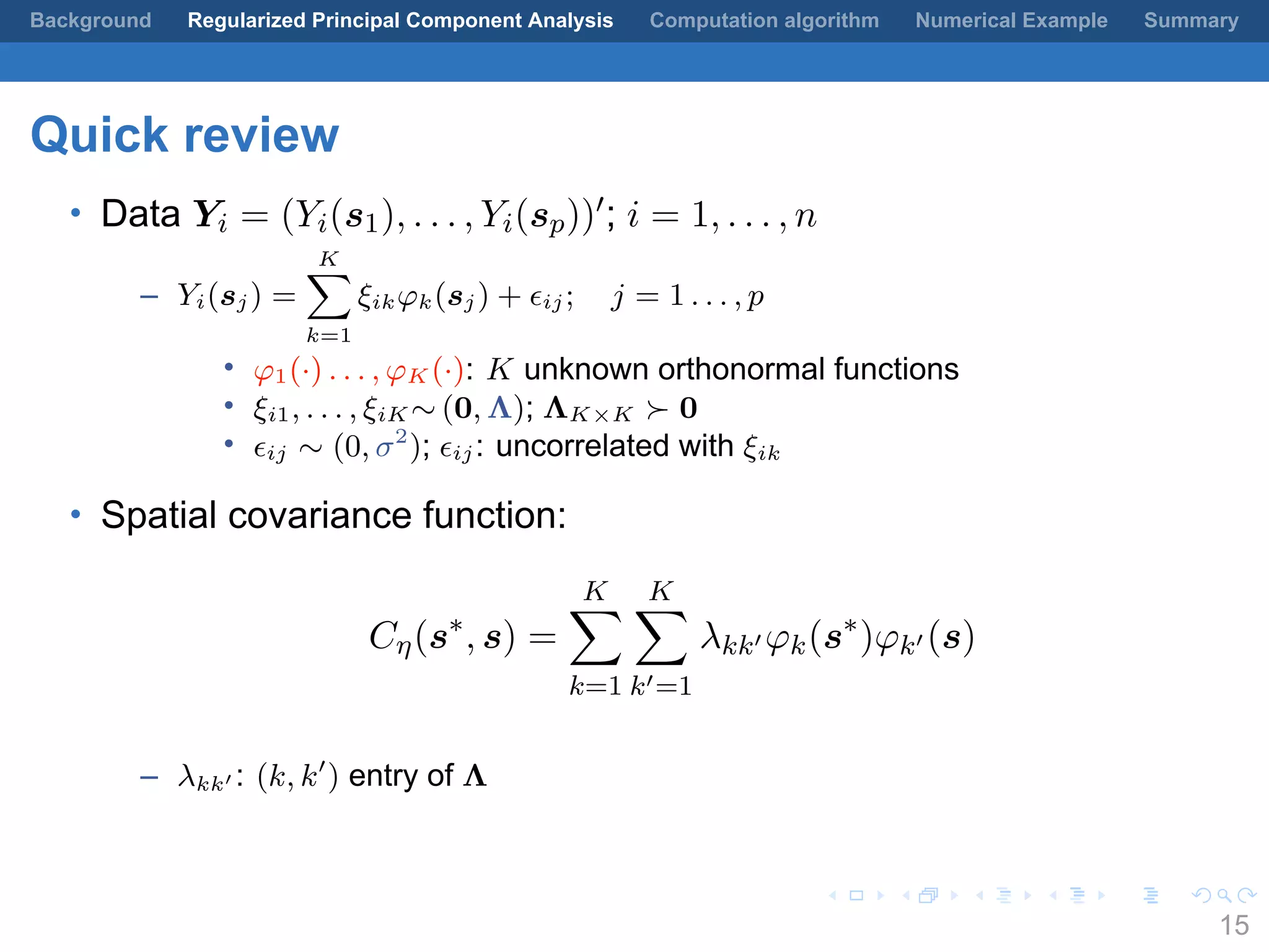
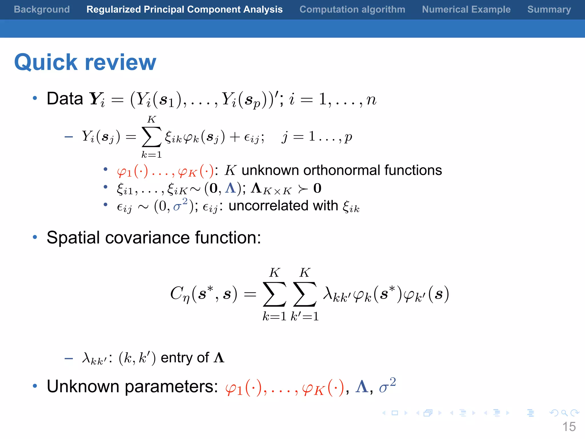
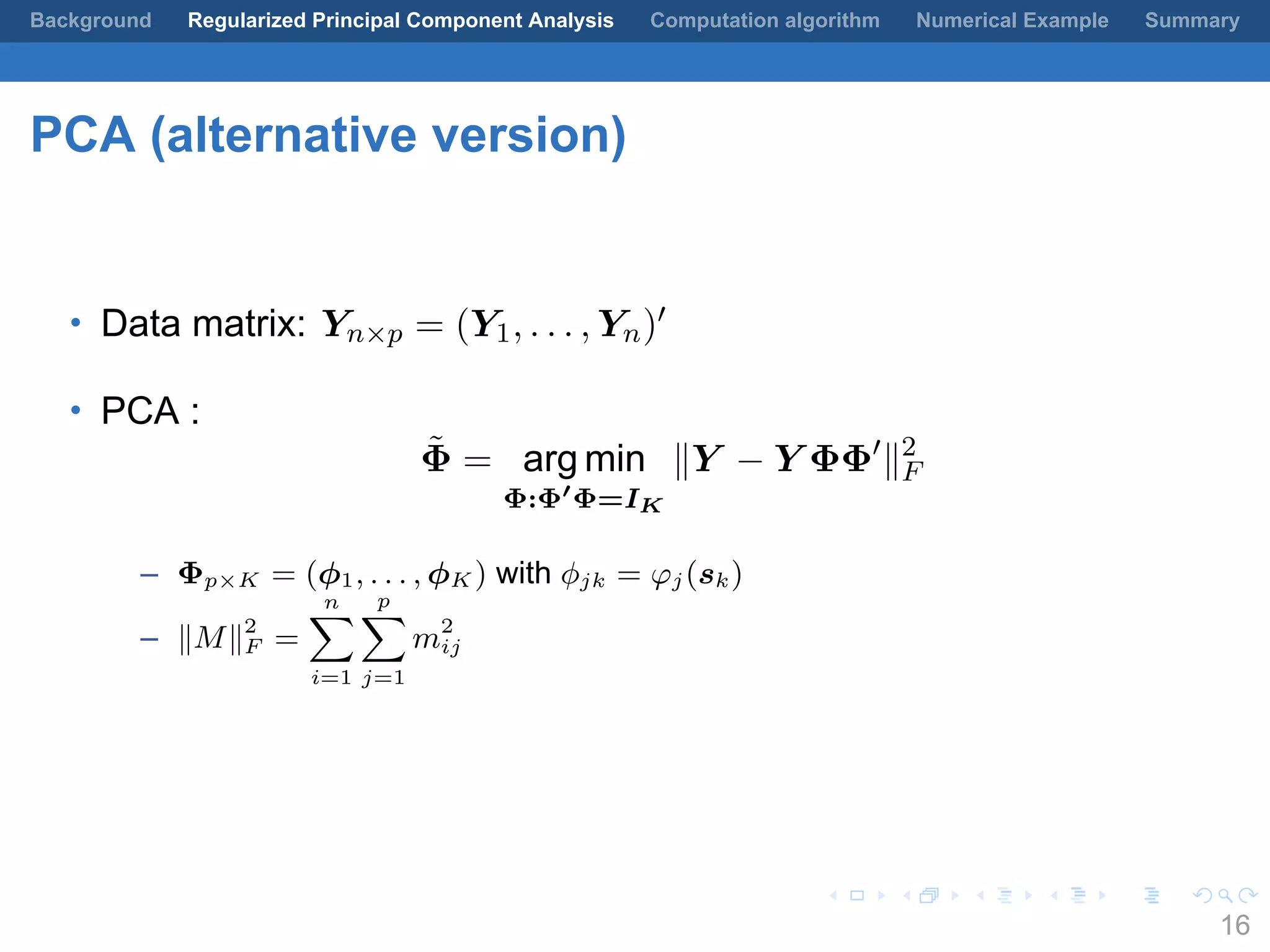
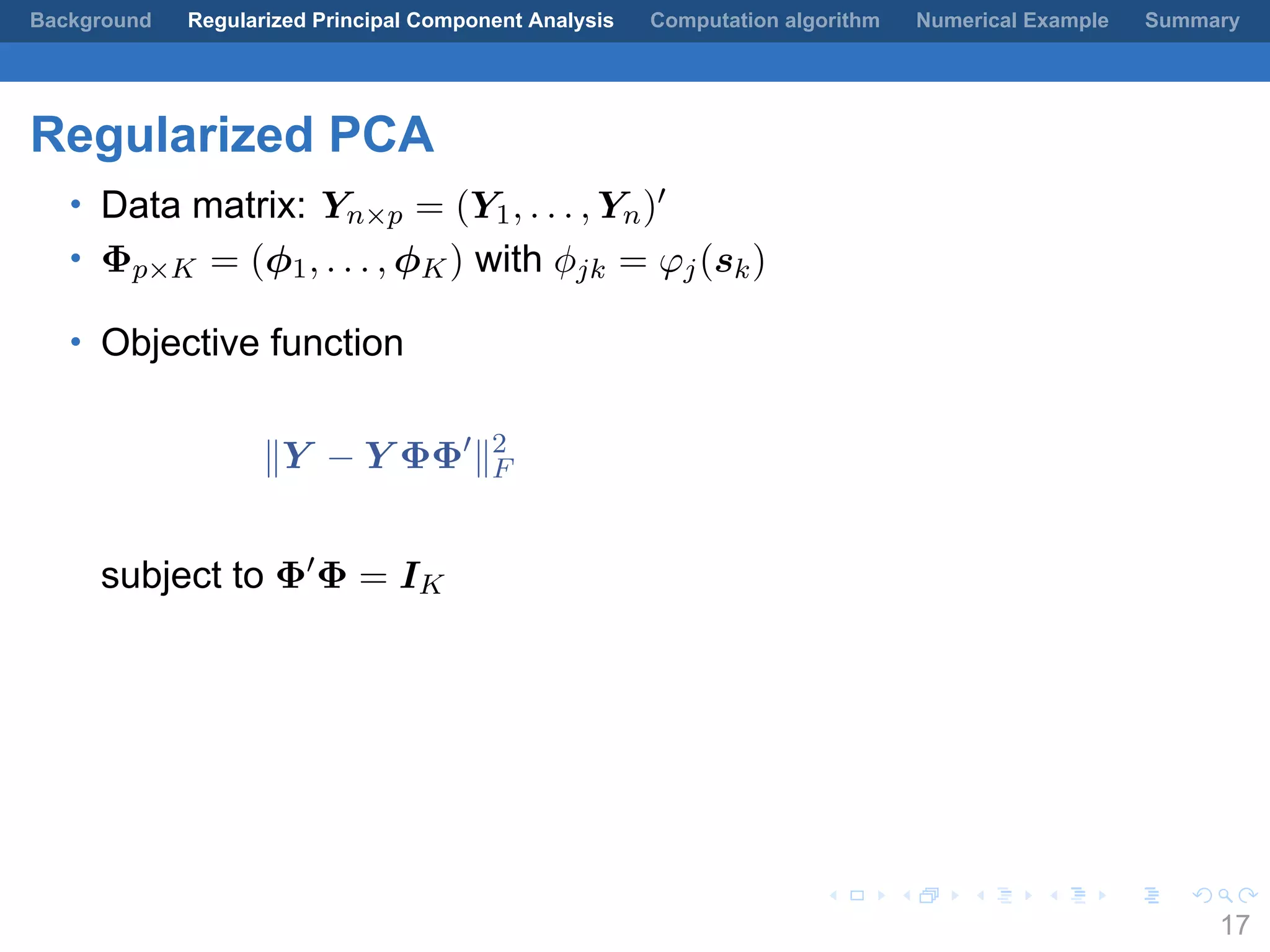
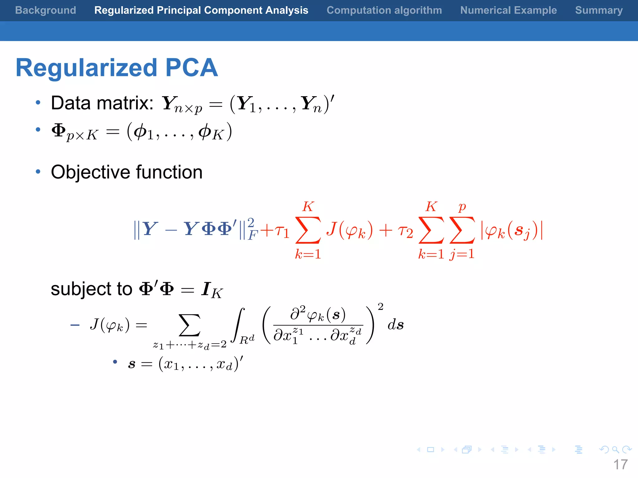
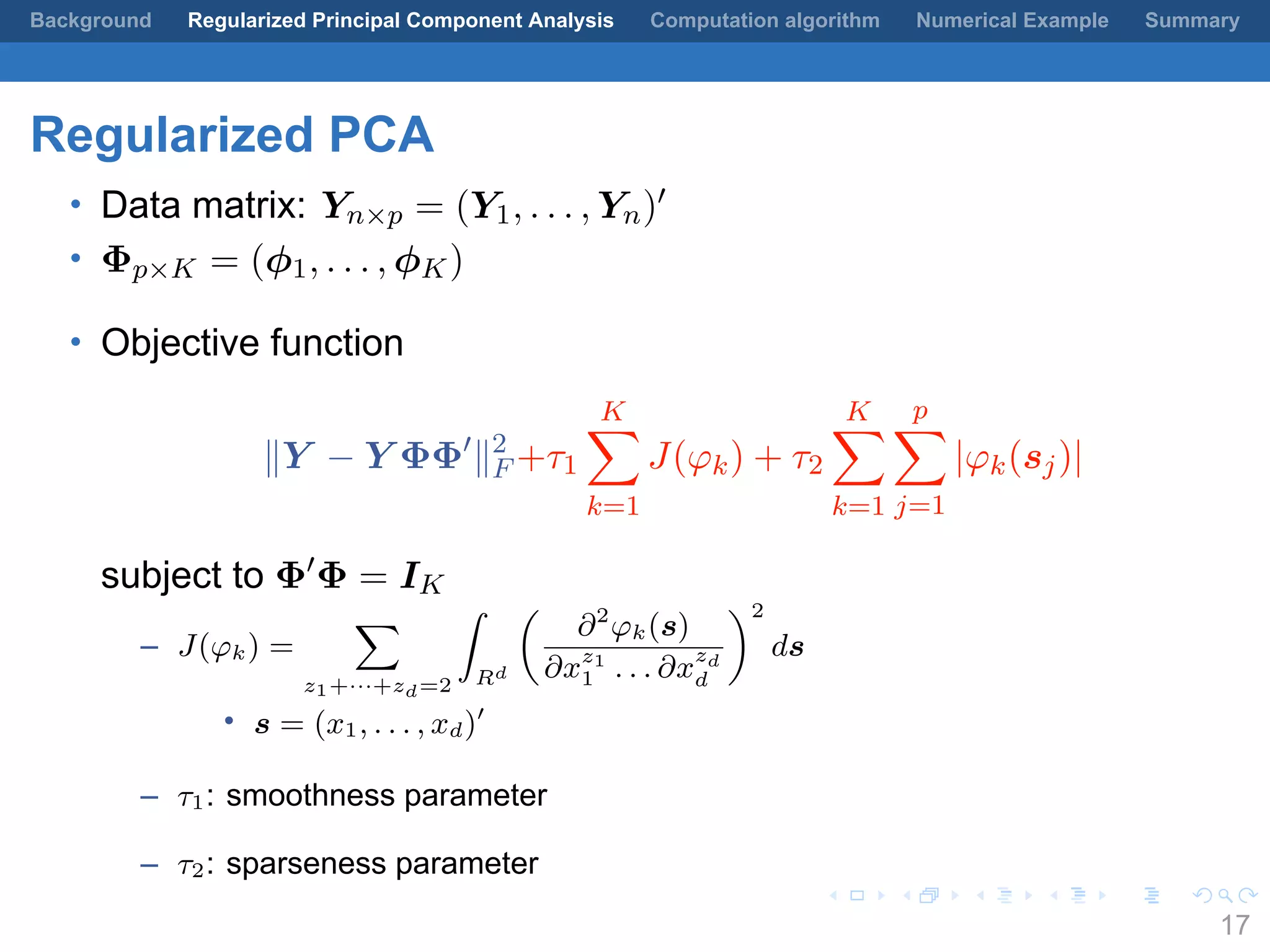
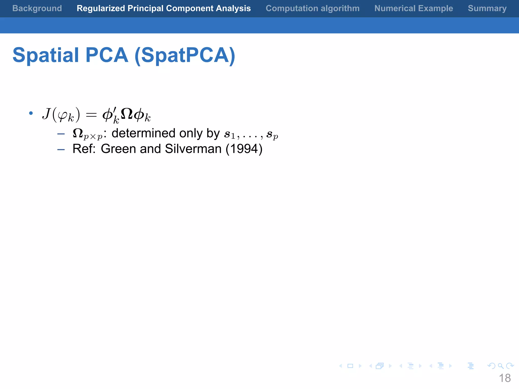
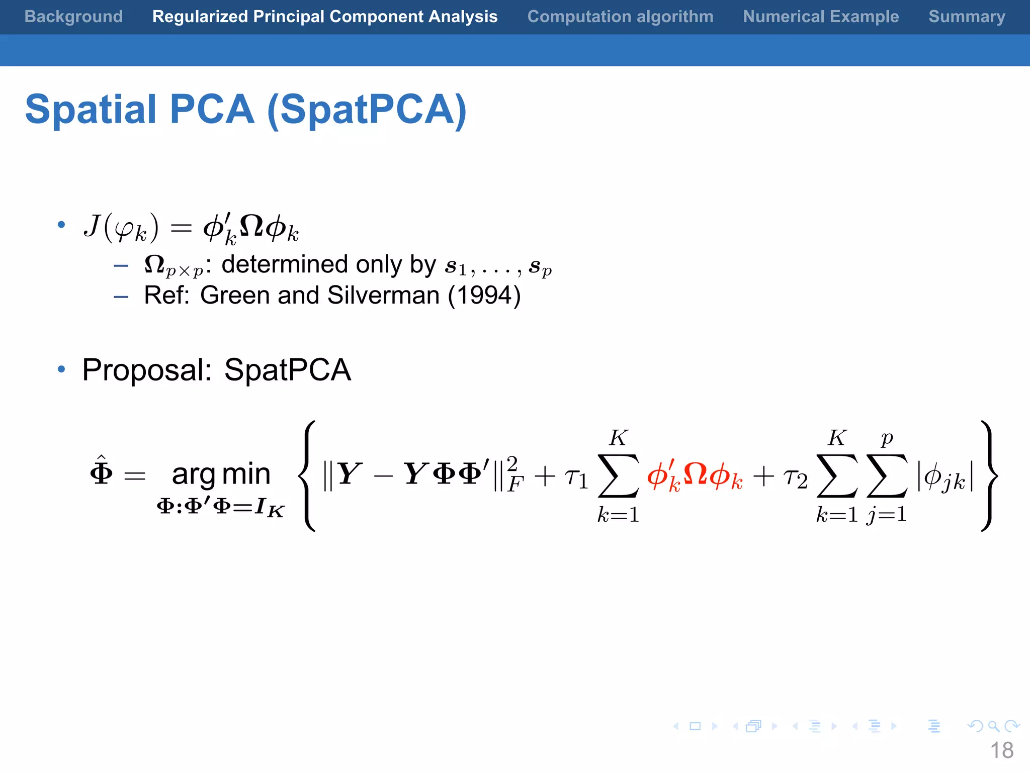
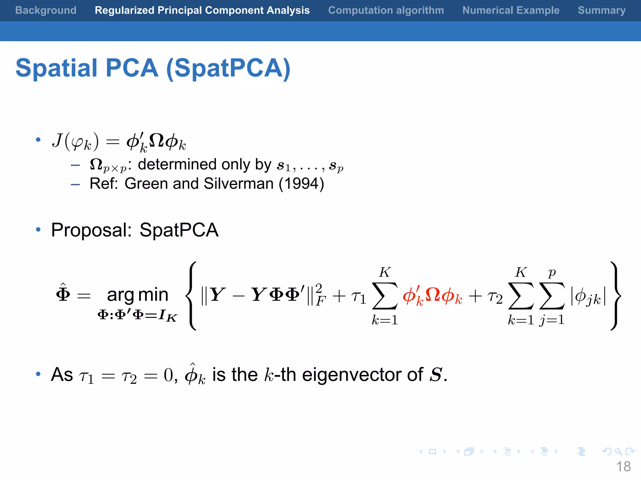
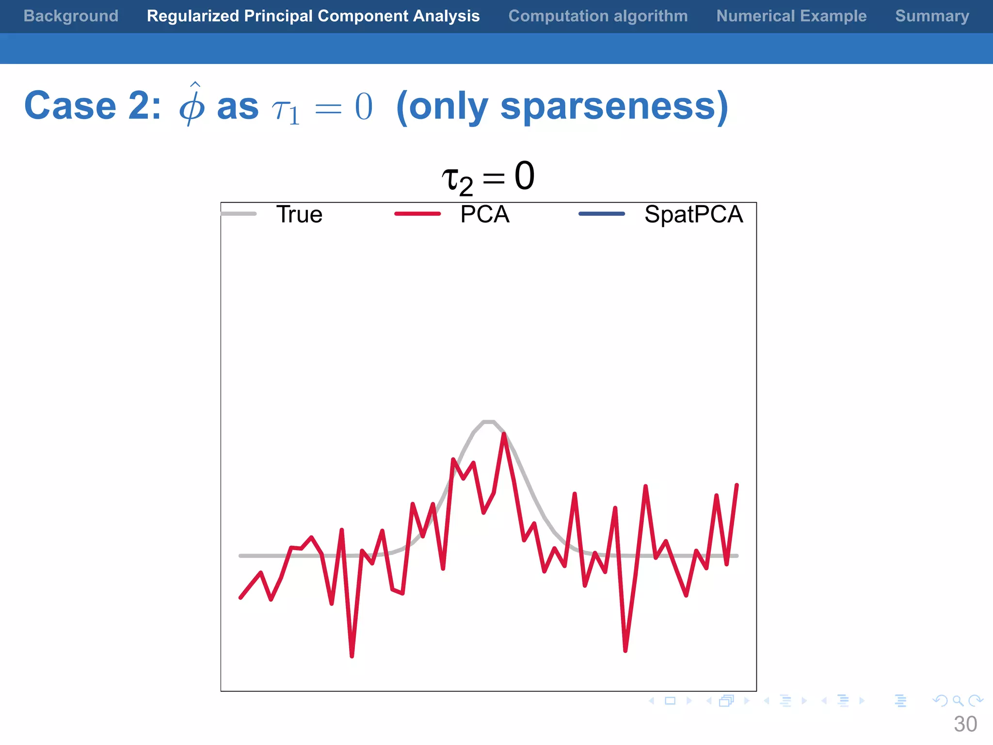
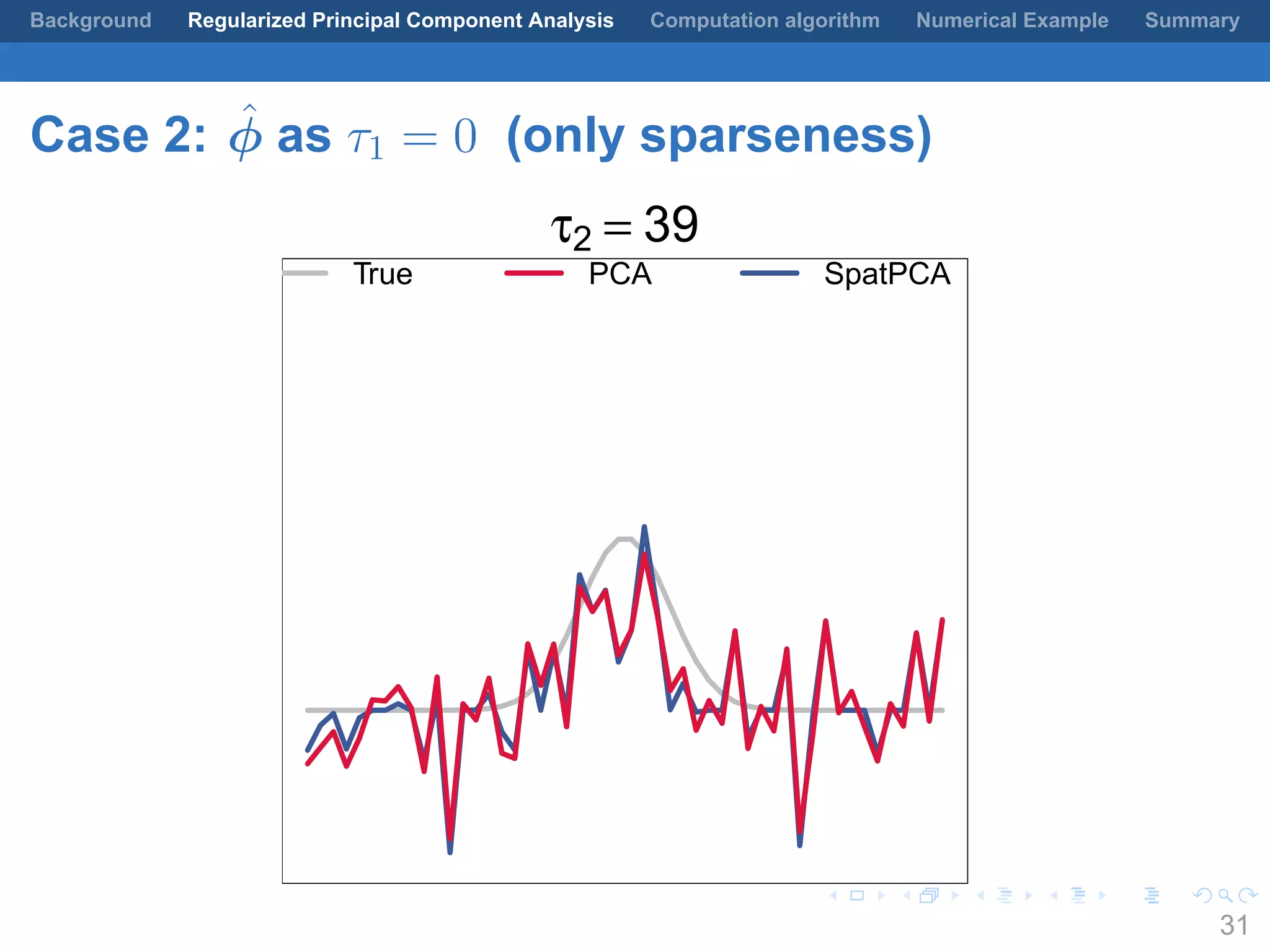
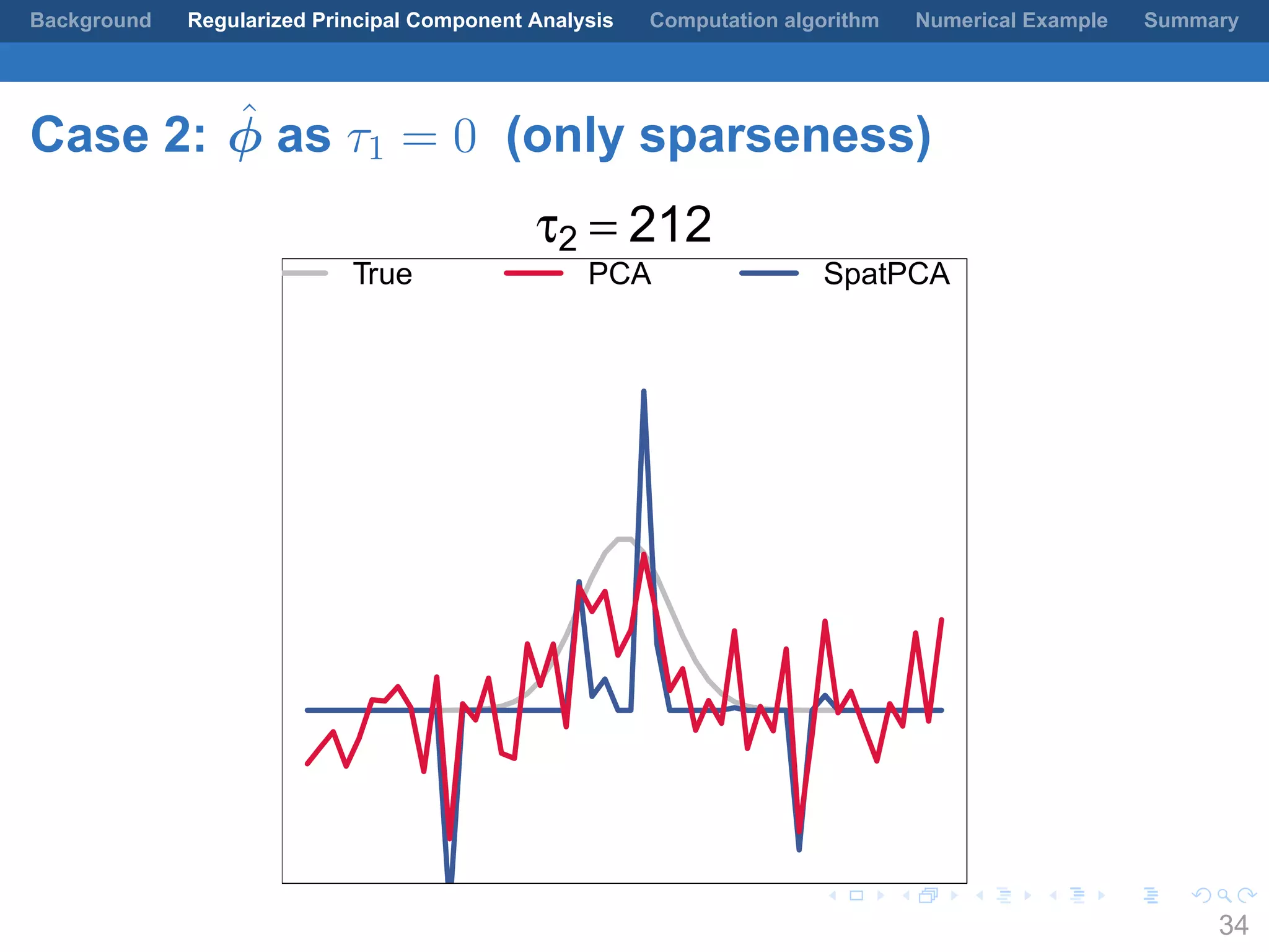
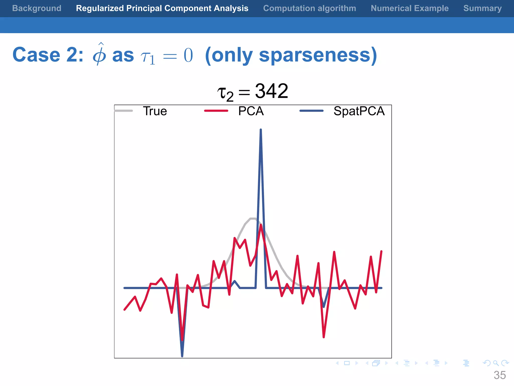
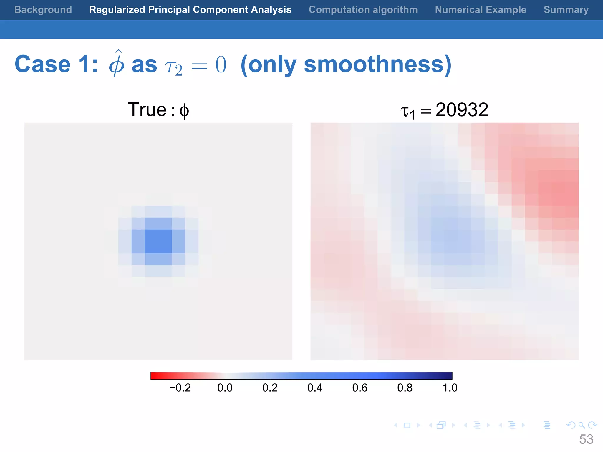
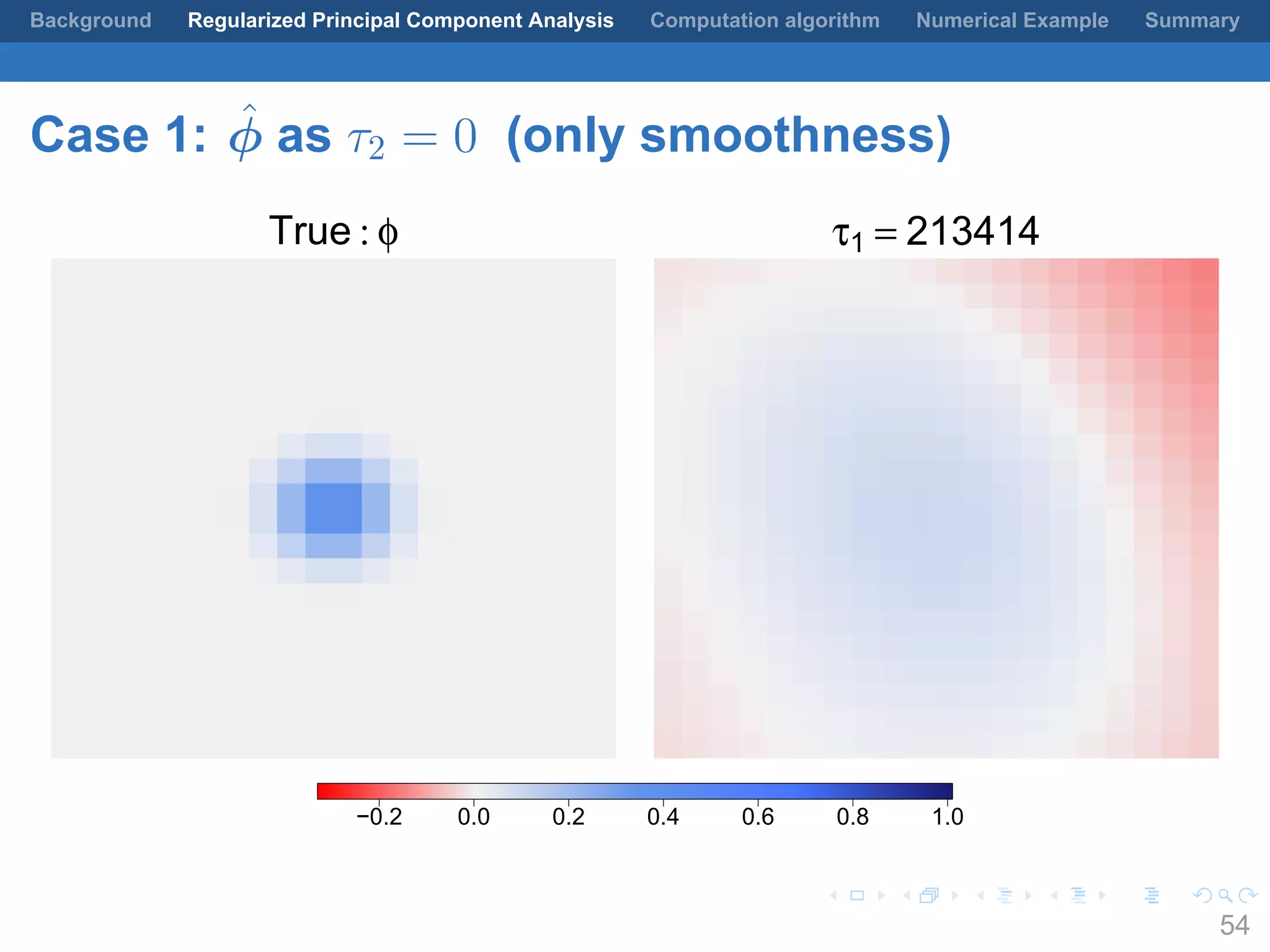
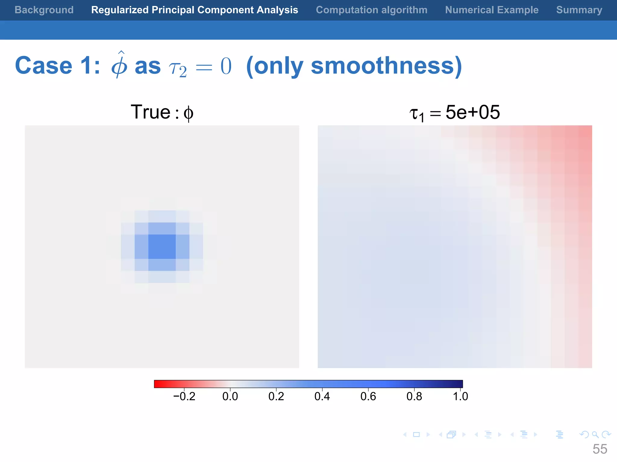
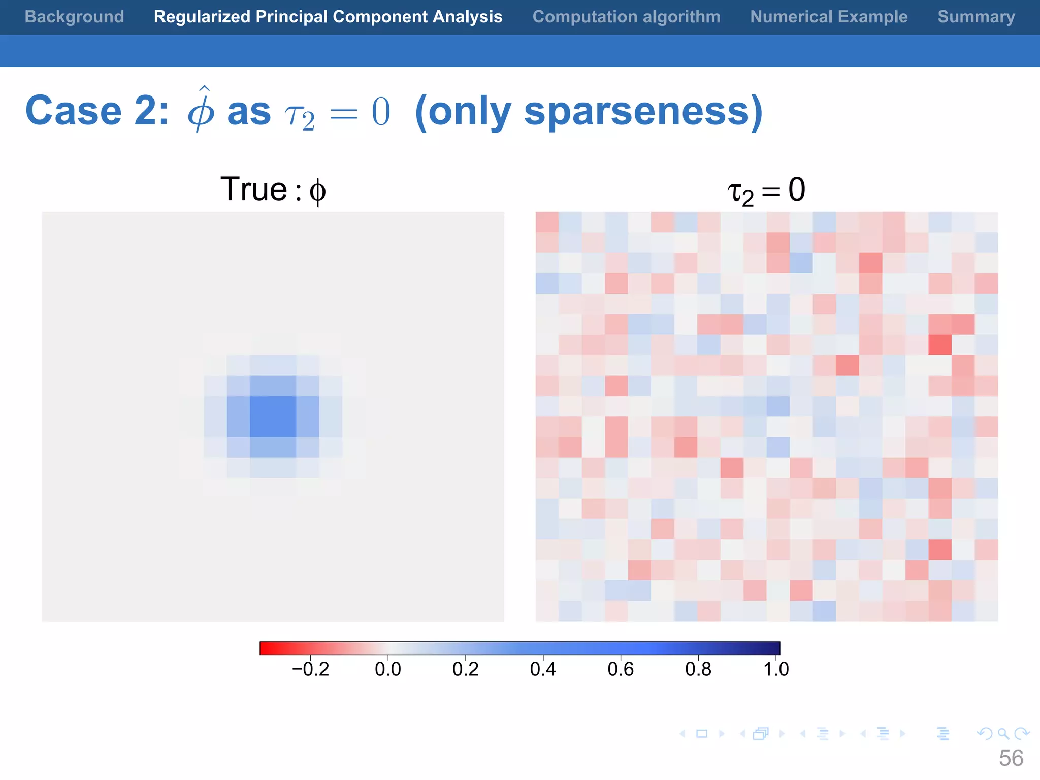
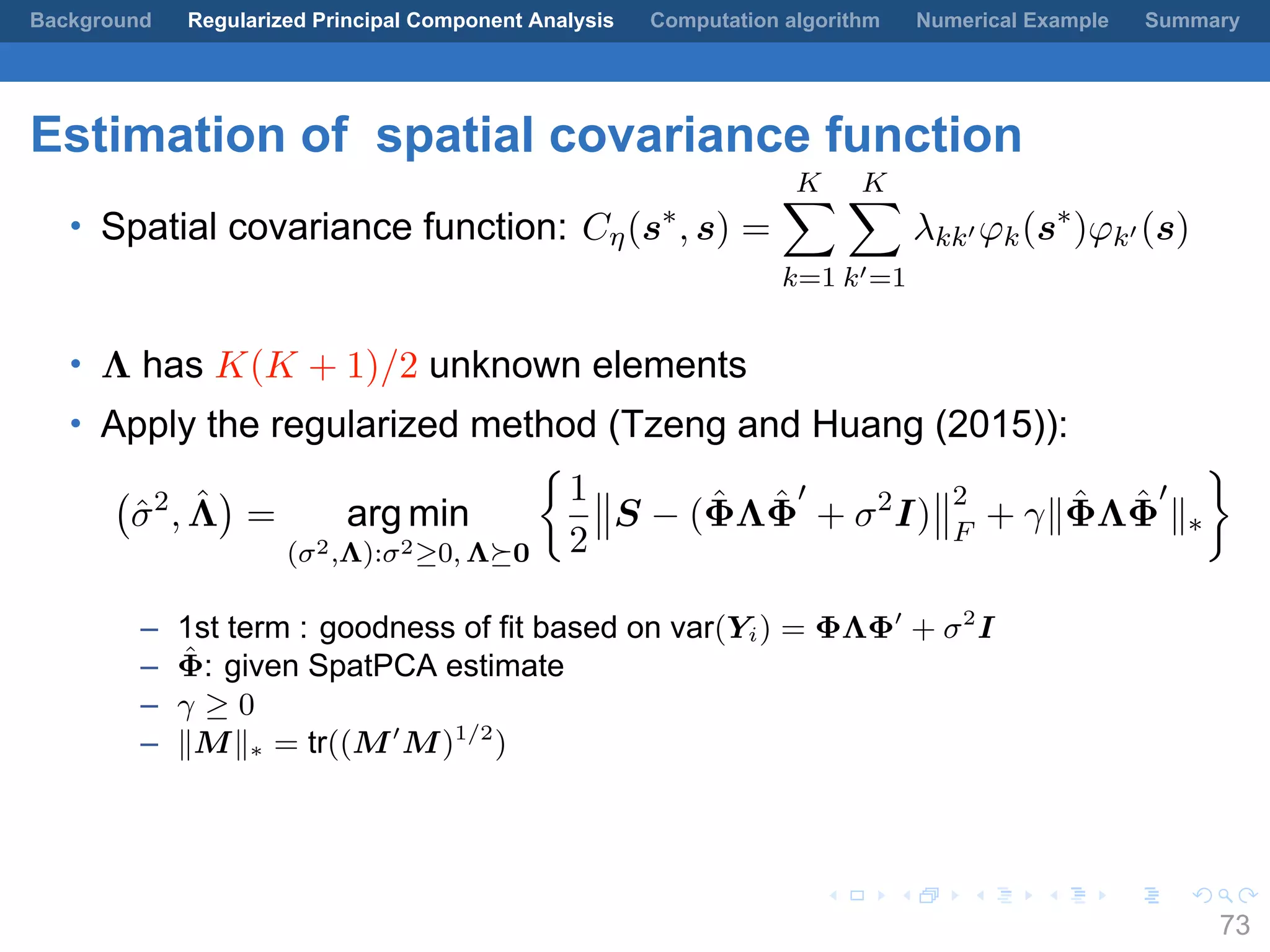
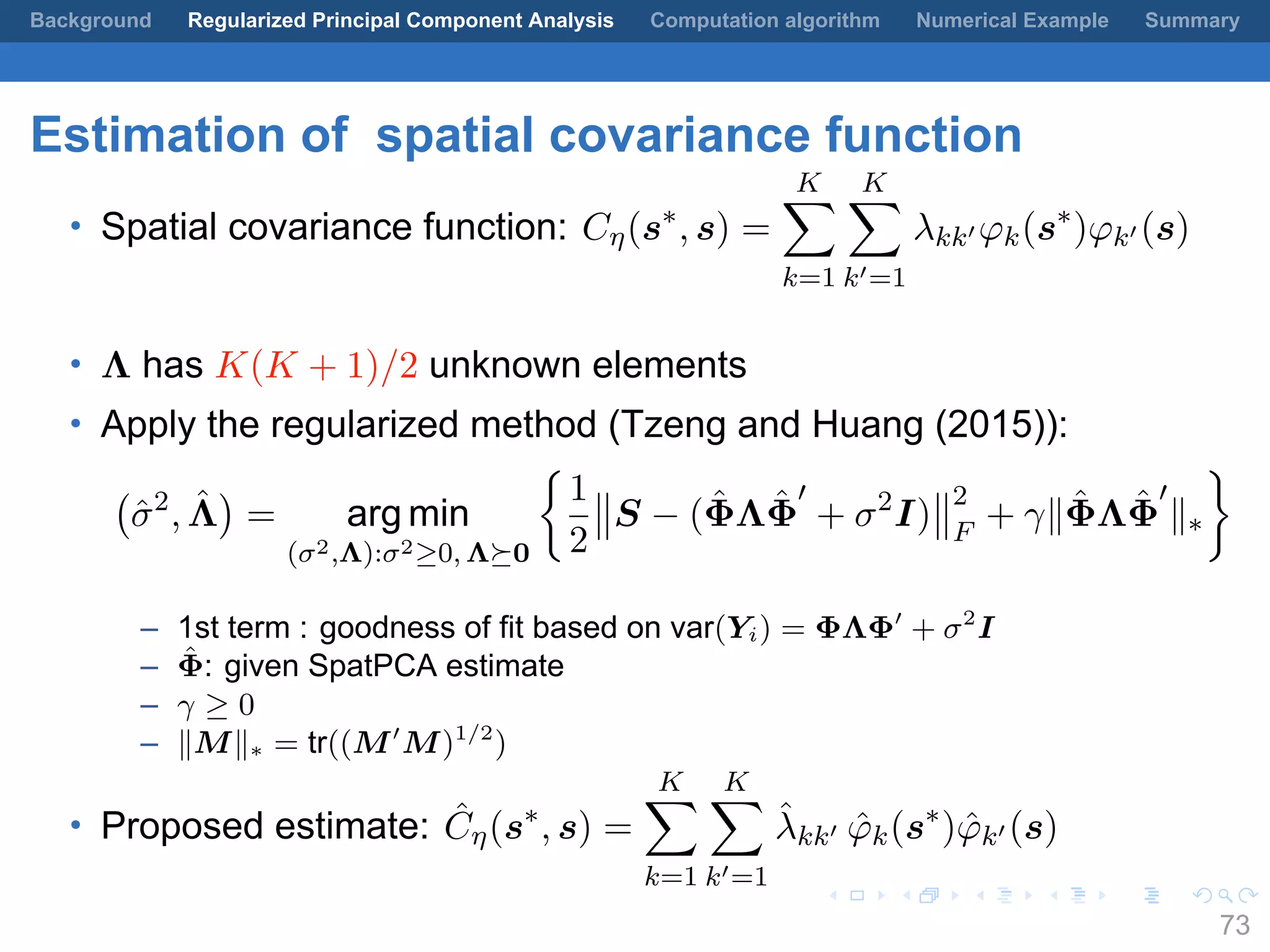
Regularized Principal Component Analysis for Spatial Data

.
.
.
.
.
.
.
.
.
.
.
.
.
.
.
.
.
.
.
.
.
.
.
.
.
.
.
.
.
.
.
.
.
.
.
.
.
.
.
.
Regularized Principal Component Analysis for
Spatial Data
Wen-Ting Wang
Institute of Statistics, National Chiao Tung University
January 25, 2017
Joint work with Hsin-Cheng Huang, Academia Sinica
1

.
.
.
.
.
.
.
.
.
.
.
.
.
.
.
.
.
.
.
.
.
.
.
.
.
.
.
.
.
.
.
.
.
.
.
.
.
.
.
.
Background Regularized Principal Component Analysis Computation algorithm Numerical Example Summary
Outline
1 Background
2 Regularized Principal Component Analysis
3 Computation algorithm
4 Numerical Example
5 Summary
2

.
.
.
.
.
.
.
.
.
.
.
.
.
.
.
.
.
.
.
.
.
.
.
.
.
.
.
.
.
.
.
.
.
.
.
.
.
.
.
.
Outline
1 Background
4 Numerical Example
5 Summary
3

.
.
.
.
.
.
.
.
.
.
.
.
.
.
.
.
.
.
.
.
.
.
.
.
.
.
.
.
.
.
.
.
.
.
.
.
.
.
.
.
Background
• Spatial processes of interest:
{ηi(s); s ∈ D} ; i = 1, . . . , n
– D ⊂ Rd
– mean zero
– common covariance function: Cη(s∗
, s) = Cov(ηi(s∗
), ηi(s))
– η1(·), . . . , ηn(·): uncorrelated
4

.
.
.
.
.
.
.
.
.
.
.
.
.
.
.
.
.
.
.
.
.
.
.
.
.
.
.
.
.
.
.
.
.
.
.
.
.
.
.
.
Background
• Spatial processes of interest:
{ηi(s); s ∈ D} ; i = 1, . . . , n
– D ⊂ Rd
– mean zero
– common covariance function: Cη(s∗
, s) = Cov(ηi(s∗
), ηi(s))
– η1(·), . . . , ηn(·): uncorrelated
• Observed data at locations s1, . . . , sp ∈ D,
Yi(sj) = ηi(sj) + ϵij; i = 1, . . . , n, j = 1, . . . , p
– ϵij ∼ (0, σ2
): white noise
– ϵij and ηi(sj) are uncorrelated for any i, j
4

.
.
.
.
.
.
.
.
.
.
.
.
.
.
.
.
.
.
.
.
.
.
.
.
.
.
.
.
.
.
.
.
.
.
.
.
.
.
.
.
Targets
1 Detect the dominant patterns (modes) of η1(·), . . . , ηn(·)
– interpret the variability of spatial data physically
2 Estimate spatial covariance function Cη(·, ·)
– no specific assumption (e.g., parametric form or stationarity)
– spatial prediction (kriging) of {ηi(s); s ∈ D}
5

.
.
.
.
.
.
.
.
.
.
.
.
.
.
.
.
.
.
.
.
.
.
.
.
.
.
.
.
.
.
.
.
.
.
.
.
.
.
.
.
Example: dominant patterns
• Two dominant patterns (Deser, 2009)
Basin-wide mode East-west dipole mode
−0.04 −0.02 0.00 0.02 0.04
– Data: Indian Ocean sea surface temperature anomalies (Monthly average)
– related to El Ninõ–Southern Oscillation (ENSO)
6

.
.
.
.
.
.
.
.
.
.
.
.
.
.
.
.
.
.
.
.
.
.
.
.
.
.
.
.
.
.
.
.
.
.
.
.
.
.
.
.
Rank-K spatial model
• Data:
Yi(sj) = ηi(sj) + ϵij; i = 1, . . . , n, j = 1 . . . , p
7

.
.
.
.
.
.
.
.
.
.
.
.
.
.
.
.
.
.
.
.
.
.
.
.
.
.
.
.
.
.
.
.
.
.
.
.
.
.
.
.
• Data:
Yi(sj) =
K∑
k=1
ξikφk(sj) + ϵij; i = 1, . . . , n, j = 1 . . . , p
– ξi1, . . . , ξiK ∼ (0, Λ); ΛK×K is positive-definite
– φ1(·) . . . , φK (·): K unknown orthonormal functions
– ξik uncorrelated with ϵij
8

.
.
.
.
.
.
.
.
.
.
.
.
.
.
.
.
.
.
.
.
.
.
.
.
.
.
.
.
.
.
.
.
.
.
.
.
.
.
.
.
• Data:
Yi(sj) =
K∑
k=1
ξikφk(sj) + ϵij; i = 1, . . . , n, j = 1 . . . , p
– ξi1, . . . , ξiK ∼ (0, Λ); ΛK×K is positive-definite
– φ1(·) . . . , φK (·): K unknown orthonormal functions
– ξik uncorrelated with ϵij
• Spatial covariance function:
Cη(s∗
, s) =
K∑
k=1
K∑
k′=1
λkk′ φk(s∗
)φk′ (s)
– λkk′ : (k, k′
) entry of Λ
8

.
.
.
.
.
.
.
.
.
.
.
.
.
.
.
.
.
.
.
.
.
.
.
.
.
.
.
.
.
.
.
.
.
.
.
.
.
.
.
.
Goal
• Find φ1(·), . . . , φK(·) to represent the dominant patterns.
9

.
.
.
.
.
.
.
.
.
.
.
.
.
.
.
.
.
.
.
.
.
.
.
.
.
.
.
.
.
.
.
.
.
.
.
.
.
.
.
.
Goal
• Find φ1(·), . . . , φK(·) to represent the dominant patterns.
• Standard approach: Principal component analysis (PCA)
9

.
.
.
.
.
.
.
.
.
.
.
.
.
.
.
.
.
.
.
.
.
.
.
.
.
.
.
.
.
.
.
.
.
.
.
.
.
.
.
.
Principal Component Analysis
• p-dimensional data vector:
Yi = (Yi(s1), . . . , Yi(sp))′
∼ (0, Σ)
• Idea: Find ϕ ∈ Rp with ϕ′ϕ = 1,which maximizes Var(ϕ′Yi)
10

.
.
.
.
.
.
.
.
.
.
.
.
.
.
.
.
.
.
.
.
.
.
.
.
.
.
.
.
.
.
.
.
.
.
.
.
.
.
.
.
Yi = (Yi(s1), . . . , Yi(sp))′
∼ (0, Σ)
• Spectral decomposition: Σ
– eigenvalues: λ1 ≥ · · · ≥ λp
– eigenvectors: ϕ1, . . . , ϕp
10

.
.
.
.
.
.
.
.
.
.
.
.
.
.
.
.
.
.
.
.
.
.
.
.
.
.
.
.
.
.
.
.
.
.
.
.
.
.
.
.
Yi = (Yi(s1), . . . , Yi(sp))′
∼ (0, Σ)
• Spectral decomposition: Σ
– eigenvalues: λ1 ≥ · · · ≥ λp
– eigenvectors: ϕ1, . . . , ϕp
• Dominant patterns: ϕ1, . . . , ϕK (with λ1, . . . , λK large)
10

.
.
.
.
.
.
.
.
.
.
.
.
.
.
.
.
.
.
.
.
.
.
.
.
.
.
.
.
.
.
.
.
.
.
.
.
.
.
.
.
• Data matrix: Yn×p = (Y1, . . . , Yn)′
• Sample covariance matrix: S = Y ′Y /n
• Spectral decomposition: S
– sample eigenvalues: ˜λ1 ≥ · · · ≥ ˜λp
– sample eigenvectors: ˜ϕ1, . . . , ˜ϕp
• ˜ϕ1, . . . , ˜ϕK are estimates of ϕ1, . . . , ϕK
11

.
.
.
.
.
.
.
.
.
.
.
.
.
.
.
.
.
.
.
.
.
.
.
.
.
.
.
.
.
.
.
.
.
.
.
.
.
.
.
.
• Sample covariance matrix: S = Y ′Y /n
• Spectral decomposition: S
– sample eigenvalues: ˜λ1 ≥ · · · ≥ ˜λp
– sample eigenvectors: ˜ϕ1, . . . , ˜ϕp
• ˜ϕ1, . . . , ˜ϕK are estimates of ϕ1, . . . , ϕK
• Problems:
– high estimation variability: n is small or p is large
→ unstable and noisy patterns
→ weak physical interpretation
– without spatial structure of ϕ
11

.
.
.
.
.
.
.
.
.
.
.
.
.
.
.
.
.
.
.
.
.
.
.
.
.
.
.
.
.
.
.
.
.
.
.
.
.
.
.
.
Example:
PCA : φ
~
−0.2 0.0 0.2 0.4 0.6 0.8 1.0
12

.
.
.
.
.
.
.
.
.
.
.
.
.
.
.
.
.
.
.
.
.
.
.
.
.
.
.
.
.
.
.
.
.
.
.
.
.
.
.
.
Example:
True : φ PCA : φ
~
−0.2 0.0 0.2 0.4 0.6 0.8 1.0
12

.
.
.
.
.
.
.
.
.
.
.
.
.
.
.
.
.
.
.
.
.
.
.
.
.
.
.
.
.
.
.
.
.
.
.
.
.
.
.
.
Motivation
To enhance the interpretablity, we implement PCA by incorporating
13

.
.
.
.
.
.
.
.
.
.
.
.
.
.
.
.
.
.
.
.
.
.
.
.
.
.
.
.
.
.
.
.
.
.
.
.
.
.
.
.
Motivation
1 spatial structure of eigenvectors
13

.
.
.
.
.
.
.
.
.
.
.
.
.
.
.
.
.
.
.
.
.
.
.
.
.
.
.
.
.
.
.
.
.
.
.
.
.
.
.
.
Motivation
2 sparsity of eigenvectors
13

.
.
.
.
.
.
.
.
.
.
.
.
.
.
.
.
.
.
.
.
.
.
.
.
.
.
.
.
.
.
.
.
.
.
.
.
.
.
.
.
Motivation
2 sparsity of eigenvectors
3 orthogonality of eigenvectors
13

.
.
.
.
.
.
.
.
.
.
.
.
.
.
.
.
.
.
.
.
.
.
.
.
.
.
.
.
.
.
.
.
.
.
.
.
.
.
.
.
Outline
1 Background
4 Numerical Example
5 Summary
14

.
.
.
.
.
.
.
.
.
.
.
.
.
.
.
.
.
.
.
.
.
.
.
.
.
.
.
.
.
.
.
.
.
.
.
.
.
.
.
.
Quick review
• Data Yi = (Yi(s1), . . . , Yi(sp))′; i = 1, . . . , n
– Yi(sj) =
K∑
k=1
ξikφk(sj) + ϵij; j = 1 . . . , p
• φ1(·) . . . , φK (·): K unknown orthonormal functions
• ξi1, . . . , ξiK ∼ (0, Λ); ΛK×K ≻ 0
• ϵij ∼ (0, σ2
); ϵij: uncorrelated with ξik
15

.
.
.
.
.
.
.
.
.
.
.
.
.
.
.
.
.
.
.
.
.
.
.
.
.
.
.
.
.
.
.
.
.
.
.
.
.
.
.
.
Quick review
– Yi(sj) =
K∑
k=1
ξikφk(sj) + ϵij; j = 1 . . . , p
• ξi1, . . . , ξiK ∼ (0, Λ); ΛK×K ≻ 0
• ϵij ∼ (0, σ2
Cη(s∗
, s) =
K∑
k=1
K∑
k′=1
λkk′ φk(s∗
)φk′ (s)
– λkk′ : (k, k′
) entry of Λ
15

.
.
.
.
.
.
.
.
.
.
.
.
.
.
.
.
.
.
.
.
.
.
.
.
.
.
.
.
.
.
.
.
.
.
.
.
.
.
.
.
Quick review
– Yi(sj) =
K∑
k=1
ξikφk(sj) + ϵij; j = 1 . . . , p
• ξi1, . . . , ξiK ∼ (0, Λ); ΛK×K ≻ 0
• ϵij ∼ (0, σ2
Cη(s∗
, s) =
K∑
k=1
K∑
k′=1
λkk′ φk(s∗
)φk′ (s)
– λkk′ : (k, k′
) entry of Λ
• Unknown parameters: φ1(·), . . . , φK(·), Λ, σ2
15

.
.
.
.
.
.
.
.
.
.
.
.
.
.
.
.
.
.
.
.
.
.
.
.
.
.
.
.
.
.
.
.
.
.
.
.
.
.
.
.
PCA (alternative version)
• PCA :
˜Φ = arg min
Φ:Φ′
Φ=IK
∥Y − Y ΦΦ′
∥2
F
– Φp×K = (ϕ1, . . . , ϕK ) with ϕjk = φj(sk)
– ∥M∥2
F =
n∑
i=1
p
∑
j=1
m2
ij
16

.
.
.
.
.
.
.
.
.
.
.
.
.
.
.
.
.
.
.
.
.
.
.
.
.
.
.
.
.
.
.
.
.
.
.
.
.
.
.
.
Regularized PCA
• Φp×K = (ϕ1, . . . , ϕK) with ϕjk = φj(sk)
• Objective function
∥Y − Y ΦΦ′
∥2
F
subject to Φ′
Φ = IK
17

.
.
.
.
.
.
.
.
.
.
.
.
.
.
.
.
.
.
.
.
.
.
.
.
.
.
.
.
.
.
.
.
.
.
.
.
.
.
.
.
Regularized PCA
• Φp×K = (ϕ1, . . . , ϕK)
∥Y − Y ΦΦ′
∥2
F +τ1
K∑
k=1
J(φk) + τ2
K∑
k=1
p∑
j=1
|φk(sj)|
subject to Φ′
Φ = IK
– J(φk) =
∑
z1+···+zd=2
∫
Rd
(
∂2
φk(s)
∂xz1
1 . . . ∂x
zd
d
)2
ds
• s = (x1, . . . , xd)′
17

.
.
.
.
.
.
.
.
.
.
.
.
.
.
.
.
.
.
.
.
.
.
.
.
.
.
.
.
.
.
.
.
.
.
.
.
.
.
.
.
Regularized PCA
• Φp×K = (ϕ1, . . . , ϕK)
∥Y − Y ΦΦ′
∥2
F +τ1
K∑
k=1
J(φk) + τ2
K∑
k=1
p∑
j=1
|φk(sj)|
subject to Φ′
Φ = IK
– J(φk) =
∑
z1+···+zd=2
∫
Rd
(
∂2
φk(s)
∂xz1
1 . . . ∂x
zd
d
)2
ds
• s = (x1, . . . , xd)′
– τ1: smoothness parameter
– τ2: sparseness parameter
17

.
.
.
.
.
.
.
.
.
.
.
.
.
.
.
.
.
.
.
.
.
.
.
.
.
.
.
.
.
.
.
.
.
.
.
.
.
.
.
.
Spatial PCA (SpatPCA)
• J(φk) = ϕ′
kΩϕk
– Ωp×p: determined only by s1, . . . , sp
– Ref: Green and Silverman (1994)
18

.
.
.
.
.
.
.
.
.
.
.
.
.
.
.
.
.
.
.
.
.
.
.
.
.
.
.
.
.
.
.
.
.
.
.
.
.
.
.
.
• J(φk) = ϕ′
kΩϕk
• Proposal: SpatPCA
ˆΦ = arg min
Φ:Φ′
Φ=IK



∥Y − Y ΦΦ′
∥2
F + τ1
K∑
k=1
ϕ′
kΩϕk + τ2
K∑
k=1
p∑
j=1
|ϕjk|



18

.
.
.
.
.
.
.
.
.
.
.
.
.
.
.
.
.
.
.
.
.
.
.
.
.
.
.
.
.
.
.
.
.
.
.
.
.
.
.
.
• J(φk) = ϕ′
kΩϕk
• Proposal: SpatPCA
ˆΦ = arg min
Φ:Φ′
Φ=IK



∥Y − Y ΦΦ′
∥2
F + τ1
K∑
k=1
ϕ′
kΩϕk + τ2
K∑
k=1
p∑
j=1
|ϕjk|



• As τ1 = τ2 = 0, ˆϕk is the k-th eigenvector of S.
18

.
.
.
.
.
.
.
.
.
.
.
.
.
.
.
.
.
.
.
.
.
.
.
.
.
.
.
.
.
.
.
.
.
.
.
.
.
.
.
.
SpatPCA: ˆφ1(·), . . . , ˆφK(·)
• ( ˆφ1(·), . . . , ˆφK(·)) minimizes
∥Y − Y ΦΦ′
∥2
F +τ1
K∑
k=1
J(φk) + τ2
K∑
k=1
p∑
j=1
|φk(sj)|,
subject to Φ′
Φ = IK
• ˆφk(·): smoothing spline based on ˆϕk
ˆφk(s) =
p∑
i=1
aig(∥s − si∥) + b0 +
d∑
j=1
bjxj
– s = (x1, . . . , xd)′
– g(r) =



1
16π
r2
log r; if d = 2,
Γ(d/2 − 2)
16πd/2
r4−d
; if d = 1, 3,
– a = (a1, . . . , ap)′
and b = (b0, b1, . . . , bd)′
depend on ˆϕk
19

.
.
.
.
.
.
.
.
.
.
.
.
.
.
.
.
.
.
.
.
.
.
.
.
.
.
.
.
.
.
.
.
.
.
.
.
.
.
.
.
Why considering two penalties?
20

.
.
.
.
.
.
.
.
.
.
.
.
.
.
.
.
.
.
.
.
.
.
.
.
.
.
.
.
.
.
.
.
.
.
.
.
.
.
.
.
1D Example
τ1 = 0
True PCA SpatPCA
21

.
.
.
.
.
.
.
.
.
.
.
.
.
.
.
.
.
.
.
.
.
.
.
.
.
.
.
.
.
.
.
.
.
.
.
.
.
.
.
.
Case 1: ˆϕ as τ2 = 0 (only smoothness)
τ1 = 0
True PCA SpatPCA
22

.
.
.
.
.
.
.
.
.
.
.
.
.
.
.
.
.
.
.
.
.
.
.
.
.
.
.
.
.
.
.
.
.
.
.
.
.
.
.
.
τ1 = 0.03
True PCA SpatPCA
23

.
.
.
.
.
.
.
.
.
.
.
.
.
.
.
.
.
.
.
.
.
.
.
.
.
.
.
.
.
.
.
.
.
.
.
.
.
.
.
.
τ1 = 0.09
True PCA SpatPCA
24

.
.
.
.
.
.
.
.
.
.
.
.
.
.
.
.
.
.
.
.
.
.
.
.
.
.
.
.
.
.
.
.
.
.
.
.
.
.
.
.
τ1 = 0.32
True PCA SpatPCA
25

.
.
.
.
.
.
.
.
.
.
.
.
.
.
.
.
.
.
.
.
.
.
.
.
.
.
.
.
.
.
.
.
.
.
.
.
.
.
.
.
τ1 = 3.81
True PCA SpatPCA
26

.
.
.
.
.
.
.
.
.
.
.
.
.
.
.
.
.
.
.
.
.
.
.
.
.
.
.
.
.
.
.
.
.
.
.
.
.
.
.
.
τ1 = 156.17
True PCA SpatPCA
27

.
.
.
.
.
.
.
.
.
.
.
.
.
.
.
.
.
.
.
.
.
.
.
.
.
.
.
.
.
.
.
.
.
.
.
.
.
.
.
.
τ1 = 6405.22
True PCA SpatPCA
28

.
.
.
.
.
.
.
.
.
.
.
.
.
.
.
.
.
.
.
.
.
.
.
.
.
.
.
.
.
.
.
.
.
.
.
.
.
.
.
.
τ1 = 25000
True PCA SpatPCA
29

.
.
.
.
.
.
.
.
.
.
.
.
.
.
.
.
.
.
.
.
.
.
.
.
.
.
.
.
.
.
.
.
.
.
.
.
.
.
.
.
Case 2: ˆϕ as τ1 = 0 (only sparseness)
τ2 = 0
True PCA SpatPCA
30

.
.
.
.
.
.
.
.
.
.
.
.
.
.
.
.
.
.
.
.
.
.
.
.
.
.
.
.
.
.
.
.
.
.
.
.
.
.
.
.
τ2 = 39
True PCA SpatPCA
31

.
.
.
.
.
.
.
.
.
.
.
.
.
.
.
.
.
.
.
.
.
.
.
.
.
.
.
.
.
.
.
.
.
.
.
.
.
.
.
.
τ2 = 82
True PCA SpatPCA
32

.
.
.
.
.
.
.
.
.
.
.
.
.
.
.
.
.
.
.
.
.
.
.
.
.
.
.
.
.
.
.
.
.
.
.
.
.
.
.
.
τ2 = 126
True PCA SpatPCA
33

.
.
.
.
.
.
.
.
.
.
.
.
.
.
.
.
.
.
.
.
.
.
.
.
.
.
.
.
.
.
.
.
.
.
.
.
.
.
.
.
τ2 = 212
True PCA SpatPCA
34

.
.
.
.
.
.
.
.
.
.
.
.
.
.
.
.
.
.
.
.
.
.
.
.
.
.
.
.
.
.
.
.
.
.
.
.
.
.
.
.
τ2 = 342
True PCA SpatPCA
35

.
.
.
.
.
.
.
.
.
.
.
.
.
.
.
.
.
.
.
.
.
.
.
.
.
.
.
.
.
.
.
.
.
.
.
.
.
.
.
.
τ2 = 472
True PCA SpatPCA
36

.
.
.
.
.
.
.
.
.
.
.
.
.
.
.
.
.
.
.
.
.
.
.
.
.
.
.
.
.
.
.
.
.
.
.
.
.
.
.
.
τ2 = 520
True PCA SpatPCA
37

.
.
.
.
.
.
.
.
.
.
.
.
.
.
.
.
.
.
.
.
.
.
.
.
.
.
.
.
.
.
.
.
.
.
.
.
.
.
.
.
Case 3: ˆϕ as τ1 = τ2
τ1 = τ2 = 0
True PCA SpatPCA
38

.
.
.
.
.
.
.
.
.
.
.
.
.
.
.
.
.
.
.
.
.
.
.
.
.
.
.
.
.
.
.
.
.
.
.
.
.
.
.
.
τ1 = τ2 = 0.02
True PCA SpatPCA
39

.
.
.
.
.
.
.
.
.
.
.
.
.
.
.
.
.
.
.
.
.
.
.
.
.
.
.
.
.
.
.
.
.
.
.
.
.
.
.
.
τ1 = τ2 = 0.04
True PCA SpatPCA
40

.
.
.
.
.
.
.
.
.
.
.
.
.
.
.
.
.
.
.
.
.
.
.
.
.
.
.
.
.
.
.
.
.
.
.
.
.
.
.
.
τ1 = τ2 = 0.09
True PCA SpatPCA
41

.
.
.
.
.
.
.
.
.
.
.
.
.
.
.
.
.
.
.
.
.
.
.
.
.
.
.
.
.
.
.
.
.
.
.
.
.
.
.
.
τ1 = τ2 = 0.41
True PCA SpatPCA
42

.
.
.
.
.
.
.
.
.
.
.
.
.
.
.
.
.
.
.
.
.
.
.
.
.
.
.
.
.
.
.
.
.
.
.
.
.
.
.
.
τ1 = τ2 = 4.19
True PCA SpatPCA
43

.
.
.
.
.
.
.
.
.
.
.
.
.
.
.
.
.
.
.
.
.
.
.
.
.
.
.
.
.
.
.
.
.
.
.
.
.
.
.
.
τ1 = τ2 = 42.68
True PCA SpatPCA
44

.
.
.
.
.
.
.
.
.
.
.
.
.
.
.
.
.
.
.
.
.
.
.
.
.
.
.
.
.
.
.
.
.
.
.
.
.
.
.
.
τ1 = τ2 = 100
True PCA SpatPCA
45

.
.
.
.
.
.
.
.
.
.
.
.
.
.
.
.
.
.
.
.
.
.
.
.
.
.
.
.
.
.
.
.
.
.
.
.
.
.
.
.
2D Example
True : φ PCA : φ
~
−0.2 0.0 0.2 0.4 0.6 0.8 1.0
46

.
.
.
.
.
.
.
.
.
.
.
.
.
.
.
.
.
.
.
.
.
.
.
.
.
.
.
.
.
.
.
.
.
.
.
.
.
.
.
.
True : φ τ1 = 0
−0.2 0.0 0.2 0.4 0.6 0.8 1.0
47

.
.
.
.
.
.
.
.
.
.
.
.
.
.
.
.
.
.
.
.
.
.
.
.
.
.
.
.
.
.
.
.
.
.
.
.
.
.
.
.
True : φ τ1 = 0
−0.2 0.0 0.2 0.4 0.6 0.8 1.0
48

.
.
.
.
.
.
.
.
.
.
.
.
.
.
.
.
.
.
.
.
.
.
.
.
.
.
.
.
.
.
.
.
.
.
.
.
.
.
.
.
True : φ τ1 = 93
−0.2 0.0 0.2 0.4 0.6 0.8 1.0
49

.
.
.
.
.
.
.
.
.
.
.
.
.
.
.
.
.
.
.
.
.
.
.
.
.
.
.
.
.
.
.
.
.
.
.
.
.
.
.
.
True : φ τ1 = 201
−0.2 0.0 0.2 0.4 0.6 0.8 1.0
50

.
.
.
.
.
.
.
.
.
.
.
.
.
.
.
.
.
.
.
.
.
.
.
.
.
.
.
.
.
.
.
.
.
.
.
.
.
.
.
.
True : φ τ1 = 437
−0.2 0.0 0.2 0.4 0.6 0.8 1.0
51

.
.
.
.
.
.
.
.
.
.
.
.
.
.
.
.
.
.
.
.
.
.
.
.
.
.
.
.
.
.
.
.
.
.
.
.
.
.
.
.
True : φ τ1 = 2053
−0.2 0.0 0.2 0.4 0.6 0.8 1.0
52

.
.
.
.
.
.
.
.
.
.
.
.
.
.
.
.
.
.
.
.
.
.
.
.
.
.
.
.
.
.
.
.
.
.
.
.
.
.
.
.
True : φ τ1 = 20932
−0.2 0.0 0.2 0.4 0.6 0.8 1.0
53

.
.
.
.
.
.
.
.
.
.
.
.
.
.
.
.
.
.
.
.
.
.
.
.
.
.
.
.
.
.
.
.
.
.
.
.
.
.
.
.
True : φ τ1 = 213414
−0.2 0.0 0.2 0.4 0.6 0.8 1.0
54

.
.
.
.
.
.
.
.
.
.
.
.
.
.
.
.
.
.
.
.
.
.
.
.
.
.
.
.
.
.
.
.
.
.
.
.
.
.
.
.
True : φ τ1 = 5e+05
−0.2 0.0 0.2 0.4 0.6 0.8 1.0
55

.
.
.
.
.
.
.
.
.
.
.
.
.
.
.
.
.
.
.
.
.
.
.
.
.
.
.
.
.
.
.
.
.
.
.
.
.
.
.
.
True : φ τ2 = 0
−0.2 0.0 0.2 0.4 0.6 0.8 1.0
56

.
.
.
.
.
.
.
.
.
.
.
.
.
.
.
.
.
.
.
.
.
.
.
.
.
.
.
.
.
.
.
.
.
.
.
.
.
.
.
.
True : φ τ2 = 35
−0.2 0.0 0.2 0.4 0.6 0.8 1.0
57

.
.
.
.
.
.
.
.
.
.
.
.
.
.
.
.
.
.
.
.
.
.
.
.
.
.
.
.
.
.
.
.
.
.
.
.
.
.
.
.
True : φ τ2 = 42
−0.2 0.0 0.2 0.4 0.6 0.8 1.0
58

.
.
.
.
.
.
.
.
.
.
.
.
.
.
.
.
.
.
.
.
.
.
.
.
.
.
.
.
.
.
.
.
.
.
.
.
.
.
.
.
True : φ τ2 = 50
−0.2 0.0 0.2 0.4 0.6 0.8 1.0
59

.
.
.
.
.
.
.
.
.
.
.
.
.
.
.
.
.
.
.
.
.
.
.
.
.
.
.
.
.
.
.
.
.
.
.
.
.
.
.
.
True : φ τ2 = 73
−0.2 0.0 0.2 0.4 0.6 0.8 1.0
60

.
.
.
.
.
.
.
.
.
.
.
.
.
.
.
.
.
.
.
.
.
.
.
.
.
.
.
.
.
.
.
.
.
.
.
.
.
.
.
.
True : φ τ2 = 127
−0.2 0.0 0.2 0.4 0.6 0.8 1.0
61

.
.
.
.
.
.
.
.
.
.
.
.
.
.
.
.
.
.
.
.
.
.
.
.
.
.
.
.
.
.
.
.
.
.
.
.
.
.
.
.
True : φ τ2 = 220
−0.2 0.0 0.2 0.4 0.6 0.8 1.0
62

.
.
.
.
.
.
.
.
.
.
.
.
.
.
.
.
.
.
.
.
.
.
.
.
.
.
.
.
.
.
.
.
.
.
.
.
.
.
.
.
True : φ τ2 = 270
−0.2 0.0 0.2 0.4 0.6 0.8 1.0
63

.
.
.
.
.
.
.
.
.
.
.
.
.
.
.
.
.
.
.
.
.
.
.
.
.
.
.
.
.
.
.
.
.
.
.
.
.
.
.
.
True : φ τ1 = τ2 = 0
−0.2 0.0 0.2 0.4 0.6 0.8 1.0
64

.
.
.
.
.
.
.
.
.
.
.
.
.
.
.
.
.
.
.
.
.
.
.
.
.
.
.
.
.
.
.
.
.
.
.
.
.
.
.
.
True : φ τ1 = τ2 = 33
−0.2 0.0 0.2 0.4 0.6 0.8 1.0
65

.
.
.
.
.
.
.
.
.
.
.
.
.
.
.
.
.
.
.
.
.
.
.
.
.
.
.
.
.
.
.
.
.
.
.
.
.
.
.
.
True : φ τ1 = τ2 = 38
−0.2 0.0 0.2 0.4 0.6 0.8 1.0
66

.
.
.
.
.
.
.
.
.
.
.
.
.
.
.
.
.
.
.
.
.
.
.
.
.
.
.
.
.
.
.
.
.
.
.
.
.
.
.
.
True : φ τ1 = τ2 = 43
−0.2 0.0 0.2 0.4 0.6 0.8 1.0
67

.
.
.
.
.
.
.
.
.
.
.
.
.
.
.
.
.
.
.
.
.
.
.
.
.
.
.
.
.
.
.
.
.
.
.
.
.
.
.
.
True : φ τ1 = τ2 = 55
−0.2 0.0 0.2 0.4 0.6 0.8 1.0
68

.
.
.
.
.
.
.
.
.
.
.
.
.
.
.
.
.
.
.
.
.
.
.
.
.
.
.
.
.
.
.
.
.
.
.
.
.
.
.
.
True : φ τ1 = τ2 = 81
−0.2 0.0 0.2 0.4 0.6 0.8 1.0
69

.
.
.
.
.
.
.
.
.
.
.
.
.
.
.
.
.
.
.
.
.
.
.
.
.
.
.
.
.
.
.
.
.
.
.
.
.
.
.
.
True : φ τ1 = τ2 = 118
−0.2 0.0 0.2 0.4 0.6 0.8 1.0
70

.
.
.
.
.
.
.
.
.
.
.
.
.
.
.
.
.
.
.
.
.
.
.
.
.
.
.
.
.
.
.
.
.
.
.
.
.
.
.
.
True : φ τ1 = τ2 = 136
−0.2 0.0 0.2 0.4 0.6 0.8 1.0
71

.
.
.
.
.
.
.
.
.
.
.
.
.
.
.
.
.
.
.
.
.
.
.
.
.
.
.
.
.
.
.
.
.
.
.
.
.
.
.
.
(τ1, τ2) selection
• M-fold cross-validation:
CV(τ1, τ2) =
1
M
M∑
m=1
∥Y (m)
− Y (m) ˆΦ
(−m)
τ1,τ2
( ˆΦ
(−m)
τ1,τ2
)′
∥2
F
72

.
.
.
.
.
.
.
.
.
.
.
.
.
.
.
.
.
.
.
.
.
.
.
.
.
.
.
.
.
.
.
.
.
.
.
.
.
.
.
.
CV(τ1, τ2) =
1
M
M∑
m=1
∥Y (m)
− Y (m) ˆΦ
(−m)
τ1,τ2
( ˆΦ
(−m)
τ1,τ2
)′
∥2
F
– Partition {Y1, . . . , Yn} into M parts with equal (or roughly) size
– Y (m)
: the sub-matrix of Y corresponding to the m-th part
– ˆΦ
(−m)
τ1,τ2
: the estimate of Φ for (τ1, τ2) based on Y (−m)
• Y (−m)
: remaining data, i.e., Y excluding Y (m)
72

.
.
.
.
.
.
.
.
.
.
.
.
.
.
.
.
.
.
.
.
.
.
.
.
.
.
.
.
.
.
.
.
.
.
.
.
.
.
.
.
CV(τ1, τ2) =
1
M
M∑
m=1
∥Y (m)
− Y (m) ˆΦ
(−m)
τ1,τ2
( ˆΦ
(−m)
τ1,τ2
)′
∥2
F
– Partition {Y1, . . . , Yn} into M parts with equal (or roughly) size
– Y (m)
: the sub-matrix of Y corresponding to the m-th part
– ˆΦ
(−m)
τ1,τ2
: the estimate of Φ for (τ1, τ2) based on Y (−m)
• Y (−m)
: remaining data, i.e., Y excluding Y (m)
• Find τ1 and τ2 which minimize CV(τ1, τ2)
72

.
.
.
.
.
.
.
.
.
.
.
.
.
.
.
.
.
.
.
.
.
.
.
.
.
.
.
.
.
.
.
.
.
.
.
.
.
.
.
.
Estimation of spatial covariance function
• Spatial covariance function: Cη(s∗
, s) =
K∑
k=1
K∑
k′=1
λkk′ φk(s∗
)φk′ (s)
• Till now, σ2 and Λ are unknown
• Λ has K(K + 1)/2 unknown elements
73

.
.
.
.
.
.
.
.
.
.
.
.
.
.
.
.
.
.
.
.
.
.
.
.
.
.
.
.
.
.
.
.
.
.
.
.
.
.
.
.
, s) =
K∑
k=1
K∑
k′=1
λkk′ φk(s∗
)φk′ (s)
• Apply the regularized method (Tzeng and Huang (2015)):
(
ˆσ2
, ˆΛ
)
= arg min
(σ2,Λ):σ2≥0, Λ⪰0
{
1
2
S − ( ˆΦΛ ˆΦ
′
+ σ2
I)
2
F
+ γ∥ ˆΦΛ ˆΦ
′
∥∗
}
– 1st term : goodness of fit based on var(Yi) = ΦΛΦ′
+ σ2
I
– ˆΦ: given SpatPCA estimate
– γ ≥ 0
– ∥M∥∗ = tr((M′
M)1/2
)
73

.
.
.
.
.
.
.
.
.
.
.
.
.
.
.
.
.
.
.
.
.
.
.
.
.
.
.
.
.
.
.
.
.
.
.
.
.
.
.
.
, s) =
K∑
k=1
K∑
k′=1
λkk′ φk(s∗
)φk′ (s)
• Apply the regularized method (Tzeng and Huang (2015)):
(
ˆσ2
, ˆΛ
)
= arg min
(σ2,Λ):σ2≥0, Λ⪰0
{
1
2
S − ( ˆΦΛ ˆΦ
′
+ σ2
I)
2
F
+ γ∥ ˆΦΛ ˆΦ
′
∥∗
}
– 1st term : goodness of fit based on var(Yi) = ΦΛΦ′
+ σ2
I
– ˆΦ: given SpatPCA estimate
– γ ≥ 0
– ∥M∥∗ = tr((M′
M)1/2
)
• Proposed estimate: ˆCη(s∗
, s) =
K∑
k=1
K∑
k′=1
ˆλkk′ ˆφk(s∗
) ˆφk′ (s)
73

.
.
.
.
.
.
.
.
.
.
.
.
.
.
.
.
.
.
.
.
.
.
.
.
.
.
.
.
.
.
.
.
.
.
.
.
.
.
.
.
Solution of (σ2
, Λ)
Closed-form solutions :
• ˆΛ = ˆV diag
(
ˆλ∗
1, . . . , ˆλ∗
K
)
ˆV ′
• ˆσ2 =



1
p − ˆL
(
tr(S) −
ˆL∑
k=1
(
ˆdk − γ
)
)
; if ˆd1 > γ,
1
p
(tr(S)) ; if ˆd1 ≤ γ ,
– ˆV diag( ˆd1, . . . , ˆdK ) ˆV ′
is the eigen-decomposition of ˆΦ
′
S ˆΦ with
ˆd1 ≥ · · · ≥ ˆdK
– ˆL = max
{
L : ˆdL − γ > 1
p−L
(
tr(S) −
∑L
k=1( ˆdk − γ)
)
, L = 1, . . . , K
}
– ˆλ∗
k = max( ˆdk − ˆσ2
− γ, 0); k = 1, . . . , K.
74

.
.
.
.
.
.
.
.
.
.
.
.
.
.
.
.
.
.
.
.
.
.
.
.
.
.
.
.
.
.
.
.
.
.
.
.
.
.
.
.
γ selection
Selection of γ by minimizing the CV criterion:
CV2(γ) =
1
M
M∑
m=1
S(m)
− ˆΦ ˆΛ
(−m)
γ
ˆΦ
′
− (ˆσ2
γ)(−m)
I
2
F
• Partition Y into M parts, Y (1), . . . , Y (M)
• S(m): sample covariance matrix associated with Y (m)
• Y (−m): remaining data
•
((
ˆσ2
γ
)(−m)
, ˆΛ
(−m)
γ
)
: estimate of (σ2, Λ) based on Y (−m)
75

.
.
.
.
.
.
.
.
.
.
.
.
.
.
.
.
.
.
.
.
.
.
.
.
.
.
.
.
.
.
.
.
.
.
.
.
.
.
.
.
Outline
1 Background
4 Numerical Example
5 Summary
76

.
.
.
.
.
.
.
.
.
.
.
.
.
.
.
.
.
.
.
.
.
.
.
.
.
.
.
.
.
.
.
.
.
.
.
.
.
.
.
.
Computation
• Original optimization problem
min
Φ
∥Y − Y ΦΦ′
∥2
F + τ1
K∑
k=1
ϕ′
iΩϕk + τ2
K∑
k=1
p∑
j=1
|ϕjk|,
subject to Φ′
Φ = IK
• Difficulties: orthogonal constraint and ℓ1 norm penalty
77

.
.
.
.
.
.
.
.
.
.
.
.
.
.
.
.
.
.
.
.
.
.
.
.
.
.
.
.
.
.
.
.
.
.
.
.
.
.
.
.
Computation
• Original optimization problem
min
Φ
∥Y − Y ΦΦ′
∥2
F + τ1
K∑
k=1
ϕ′
iΩϕk + τ2
K∑
k=1
p∑
j=1
|ϕjk|,
subject to Φ′
Φ = IK
• Difficulties: orthogonal constraint and ℓ1 norm penalty
• Alternating direction method of multipliers (ADMM)
– Gabay and Mercier (1976), Boyd, et. al. (2010).
– Idea: original optimization problem → several easy subproblems
77

.
.
.
.
.
.
.
.
.
.
.
.
.
.
.
.
.
.
.
.
.
.
.
.
.
.
.
.
.
.
.
.
.
.
.
.
.
.
.
.
Alternating direction method of multipliers
• Equivalent problem (ADMM form):
min
Φ,Q,R
∥Y − Y ΦΦ′
∥2
F + τ1
K∑
k=1
ϕ′
iΩϕk + τ2
K∑
k=1
p∑
j=1
|rjk| ,
subject to Q′Q = IK and Φ = Q = R
78

.
.
.
.
.
.
.
.
.
.
.
.
.
.
.
.
.
.
.
.
.
.
.
.
.
.
.
.
.
.
.
.
.
.
.
.
.
.
.
.
Alternating direction method of multipliers
• Equivalent problem (ADMM form):
min
Φ,Q,R
∥Y − Y ΦΦ′
∥2
F + τ1
K∑
k=1
ϕ′
iΩϕk + τ2
K∑
k=1
p∑
j=1
|rjk| ,
subject to Q′Q = IK and Φ = Q = R
• Augmented Lagrangian function:
L(Φ, Q, R, Γ1, Γ2)
=∥Y − Y ΦΦ′
∥2
F + τ1
K∑
k=1
ϕ′
iΩϕk + τ2
K∑
k=1
p∑
j=1
|rjk|
+ tr(Γ′
2(Φ − R)) +
ρ
2
∥Φ − R∥2
F
+ tr(Γ′
1(Φ − Q)) +
ρ
2
∥Φ − Q∥2
F subject to Q′Q = IK
– Γ1, Γ2:Lagrange multipliers; some ρ > 0
78

.
.
.
.
.
.
.
.
.
.
.
.
.
.
.
.
.
.
.
.
.
.
.
.
.
.
.
.
.
.
.
.
.
.
.
.
.
.
.
.
Algorithm:at the ℓ-th iteration
Φ(ℓ+1)
= arg min
Φ
L
(
Φ, Q(ℓ)
, R(ℓ)
, Γ
(ℓ)
1 , Γ
(ℓ)
2
)
Q(ℓ+1)
= arg min
Q:Q′Q=IK
L
(
Φ(ℓ+1)
, Q, R(ℓ)
Γ
(ℓ)
1 , Γ
(ℓ)
2
)
R(ℓ+1)
= arg min
R
L
(
Φ(ℓ+1)
, Q(ℓ+1)
, R, Γ
(ℓ)
1 , Γ
(ℓ)
2
)
Γ
(ℓ+1)
1 = Γ
(ℓ)
1 + ρ
(
Φ(ℓ+1)
− Q(ℓ+1)
)
Γ
(ℓ+1)
2 = Γ
(ℓ)
2 + ρ
(
Φ(ℓ+1)
− R(ℓ+1)
)
79

.
.
.
.
.
.
.
.
.
.
.
.
.
.
.
.
.
.
.
.
.
.
.
.
.
.
.
.
.
.
.
.
.
.
.
.
.
.
.
.
Φ(ℓ+1)
=
1
2
(τ1Ω + ρIp − Y ′
Y )−1
{
ρ
(
Q(ℓ)
+ R(ℓ)
)
− Γ1 − Γ2
}
Q(ℓ+1)
= U(ℓ)
(
V (ℓ)
)′
R(ℓ+1)
=
1
ρ
Sτ2
(
ρΦ(ℓ+1)
+ Γ
(ℓ)
1
)
Γ
(ℓ+1)
1 = Γ
(ℓ)
1 + ρ
(
Φ(ℓ+1)
− Q(ℓ+1)
)
Γ
(ℓ+1)
2 = Γ
(ℓ)
2 + ρ
(
Φ(ℓ+1)
− R(ℓ+1)
)
• U(ℓ)D(ℓ)
(
V (ℓ)
)′
= Φ(ℓ+1)
+
1
ρ
Γ
(ℓ)
2 (SVD)
• Sτ (S) = {sign(sik) max(|sik| − τ, 0)}
80

.
.
.
.
.
.
.
.
.
.
.
.
.
.
.
.
.
.
.
.
.
.
.
.
.
.
.
.
.
.
.
.
.
.
.
.
.
.
.
.
Φ(ℓ+1)
=
1
2
(τ1Ω + ρIp − Y ′
Y )−1
{
ρ
(
Q(ℓ)
+ R(ℓ)
)
− Γ1 − Γ2
}
Q(ℓ+1)
= U(ℓ)
(
V (ℓ)
)′
R(ℓ+1)
=
1
ρ
Sτ2
(
ρΦ(ℓ+1)
+ Γ
(ℓ)
1
)
Γ
(ℓ+1)
1 = Γ
(ℓ)
1 + ρ
(
Φ(ℓ+1)
− Q(ℓ+1)
)
Γ
(ℓ+1)
2 = Γ
(ℓ)
2 + ρ
(
Φ(ℓ+1)
− R(ℓ+1)
)
• U(ℓ)D(ℓ)
(
V (ℓ)
)′
= Φ(ℓ+1)
+
1
ρ
Γ
(ℓ)
2 (SVD)
• Sτ (S) = {sign(sik) max(|sik| − τ, 0)}
• All subproblems have closed-form solutions.
80

.
.
.
.
.
.
.
.
.
.
.
.
.
.
.
.
.
.
.
.
.
.
.
.
.
.
.
.
.
.
.
.
.
.
.
.
.
.
.
.
Outline
1 Background
4 Numerical Example
5 Summary
81

.
.
.
.
.
.
.
.
.
.
.
.
.
.
.
.
.
.
.
.
.
.
.
.
.
.
.
.
.
.
.
.
.
.
.
.
.
.
.
.
Example: Artificial Sea Surface Temperature Data
• Data settings:
Yi(sj) = ξi1φ1(sj) + ξi2φ2(sj) + ϵij;
– j = 1, . . . , p = 2780, i = 1, . . . , n = 60
– s1, . . . , s2780: located in the Indian Ocean
– ξi1 ∼ N(0, 101.7), ξi2 ∼ N(0, 17.1), cov(ξi1, ξi2) = 0
– ϵij ∼ N(0, 1)
– (τ1, τ2): selected by 5-fold CV
φ1(s) φ2(s)
−0.04 −0.02 0.00 0.02 0.04
82

.
.
.
.
.
.
.
.
.
.
.
.
.
.
.
.
.
.
.
.
.
.
.
.
.
.
.
.
.
.
.
.
.
.
.
.
.
.
.
.
Result I: φ1(s)
True
PCA SpatPCA
−0.04 −0.02 0.00 0.02 0.04
83

.
.
.
.
.
.
.
.
.
.
.
.
.
.
.
.
.
.
.
.
.
.
.
.
.
.
.
.
.
.
.
.
.
.
.
.
.
.
.
.
Result I: φ2(s)
True
PCA SpatPCA
−0.04 −0.02 0.00 0.02 0.04
84

.
.
.
.
.
.
.
.
.
.
.
.
.
.
.
.
.
.
.
.
.
.
.
.
.
.
.
.
.
.
.
.
.
.
.
.
.
.
.
.
Result II: Performance
• Loss function: Loss( ˆCη) =
p∑
i=1
p∑
j=1
(
ˆCη(si, sj) − Cη(si, sj)
)2
• 50 replications
– γ: selected by 5-fold CV
85

.
.
.
.
.
.
.
.
.
.
.
.
.
.
.
.
.
.
.
.
.
.
.
.
.
.
.
.
.
.
.
.
.
.
.
.
.
.
.
.
Result II: Performance
• Loss function: Loss( ˆCη) =
p∑
i=1
p∑
j=1
(
ˆCη(si, sj) − Cη(si, sj)
)2
• 50 replications
– γ: selected by 5-fold CV
• Boxplot:
q
q
q
0
5000
10000
15000
PCA SpatPCA
85

.
.
.
.
.
.
.
.
.
.
.
.
.
.
.
.
.
.
.
.
.
.
.
.
.
.
.
.
.
.
.
.
.
.
.
.
.
.
.
.
Example: 8-hour average ozone data
• Region: midwestern US
• Number of effective sites: 67 (irregular locations)
• Number of time points: 89 days (June 3 through August 31, 1987)
• At each sites, time-series is linearly detrended
−93 −83
3744
longitude
latitude
illinois indiana
iowa
kentucky
michigan:south
missouri
ohio
wisconsin
86

.
.
.
.
.
.
.
.
.
.
.
.
.
.
.
.
.
.
.
.
.
.
.
.
.
.
.
.
.
.
.
.
.
.
.
.
.
.
.
.
Result I: φ1(s)
PCA + interpolation SpatPCA
0.00 0.05 0.10 0.15 0.20
87

.
.
.
.
.
.
.
.
.
.
.
.
.
.
.
.
.
.
.
.
.
.
.
.
.
.
.
.
.
.
.
.
.
.
.
.
.
.
.
.
Outline
1 Background
4 Numerical Example
5 Summary
88

.
.
.
.
.
.
.
.
.
.
.
.
.
.
.
.
.
.
.
.
.
.
.
.
.
.
.
.
.
.
.
.
.
.
.
.
.
.
.
.
Summary
SpatPCA:
• higher-dimensional analysis → (low-dimensional) structure
• with the smoothness and sparseness penalties
• enhance physical interpretation
89

.
.
.
.
.
.
.
.
.
.
.
.
.
.
.
.
.
.
.
.
.
.
.
.
.
.
.
.
.
.
.
.
.
.
.
.
.
.
.
.
Summary
SpatPCA:
• non-stationary spatial covariance function
• can cope with irregular locations
89

.
.
.
.
.
.
.
.
.
.
.
.
.
.
.
.
.
.
.
.
.
.
.
.
.
.
.
.
.
.
.
.
.
.
.
.
.
.
.
.
Summary
SpatPCA:
• non-stationary spatial covariance function
• can cope with irregular locations
• simple and efficient algorithm
• R package: SpatPCA
– CRAN: https://cran.r-project.org/web/packages/SpatPCA/index.html
– GitHub: https://github.com/egpivo/SpatPCA
89

.
.
.
.
.
.
.
.
.
.
.
.
.
.
.
.
.
.
.
.
.
.
.
.
.
.
.
.
.
.
.
.
.
.
.
.
.
.
.
.
Thanks for your attention!
90

Regularized Principal Component Analysis for Spatial Data

More Related Content

What's hot

Viewers also liked

Similar to Regularized Principal Component Analysis for Spatial Data

Recently uploaded

Regularized Principal Component Analysis for Spatial Data