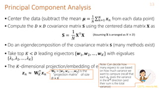
Principal Component Analysis (PCA) is a technique for dimensionality reduction that projects high-dimensional data onto a lower-dimensional space in a way that maximizes variance. It works by finding the directions (principal components) along which the variance of the data is highest. These principal components become the new axes of the reduced space. PCA involves computing the covariance matrix of the data, performing eigendecomposition on the covariance matrix to obtain its eigenvectors, and projecting the data onto the top K eigenvectors corresponding to the largest eigenvalues, where K is the target dimensionality. This projection both reduces dimensionality and maximizes retained variance.

1. Dimensionality Reduction: Principal
Component Analysis
CS771: Introduction to Machine Learning
Nisheeth

2. CS771: Intro to ML
K-means loss function: recap
2
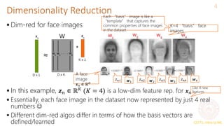
X Z
N
K
K
𝒛𝑛 = [𝑧𝑛1, 𝑧𝑛2, … , 𝑧𝑛𝐾]
denotes a length 𝐾 one-
hot encoding of 𝒙𝑛
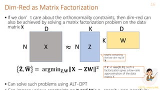
• Remember the matrix factorization view of the k-means loss function?
• We approximated an N x D matrix with
• An NxK matrix and a
• KXD matrix
• This could be storage efficient if K is much smaller than D
D
D

3. CS771: Intro to ML
Dimensionality Reduction
3
 A broad class of techniques
 Goal is to compress the original representation of the inputs
 Example: Approximate each input 𝒙𝑛 ∈ ℝ𝐷, 𝑛 = 1,2, … , 𝑁 as a linear
combination of 𝐾 < min{𝐷, 𝑁} “basis” vectors 𝒘1, 𝒘2, … , 𝒘𝐾, each
also ∈ ℝ𝐷
 We have represented each 𝒙𝑛 ∈ ℝ𝐷 by a 𝐾-dim vector 𝒛𝑛 (a new feat.
rep)
 To store 𝑁 such inputs {𝒙𝑛}𝑛=1
𝑁
, we need to keep 𝐖 and {𝒛𝑛}𝑛=1
𝑁
 Originally we required 𝑁 × 𝐷 storage, now 𝑁 × 𝐾 + 𝐷 × 𝐾 = 𝑁 + 𝐷 × 𝐾
storage
𝒙𝑛 ≈
𝑘=1
𝐾
𝑧𝑛𝑘𝒘𝑘 = 𝐖𝒛𝑛
𝐖 = 𝒘1, 𝒘2, … , 𝒘𝐾 is 𝐷 × 𝐾
𝒛𝑛 = 𝑧𝑛1, 𝑧𝑛2, … , 𝑧𝑛𝐾 is 𝐾 × 1
Note: These “basis” vectors need not
necessarily be linearly independent. But
for some dim. red. techniques, e.g.,
classic principal component analysis
(PCA), they are
Can think of W as a linear mapping
that transforms low-dim 𝒛𝑛 to high-
dim 𝒙𝑛
Some dim-red techniques assume a
nonlinear mapping function 𝑓 such that
𝒙𝑛 = 𝑓(𝒛𝑛)
For example, 𝑓 can be
modeled by a kernel or a
deep neural net

4. CS771: Intro to ML
Dimensionality Reduction
4
 Dim-red for face images
 In this example, 𝒛𝑛 ∈ ℝ𝐾 (𝐾 = 4) is a low-dim feature rep. for 𝒙𝑛 ∈ ℝ𝐷
 Essentially, each face image in the dataset now represented by just 4 real
numbers 
 Different dim-red algos differ in terms of how the basis vectors are
defined/learned
A face
image
𝒙𝑛 ∈ ℝ𝐷
K=4 “basis” face
images
Each “basis” image is like a
“template” that captures the
common properties of face images
in the dataset
𝑧𝑛1 𝑧𝑛2 𝑧𝑛3 𝑧𝑛4
𝒘1 𝒘2 𝒘3
𝒘4
+
Like 4 new
features

5. CS771: Intro to ML
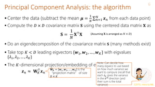
Principal Component Analysis (PCA)
5
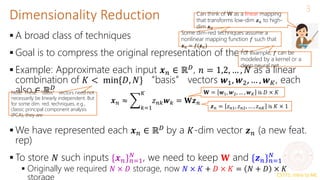
 A classic linear dim. reduction method (Pearson, 1901; Hotelling, 1930)
 Can be seen as
 Learning directions (co-ordinate axes) that capture maximum variance in data
 Learning projection directions that result in smallest reconstruction error
 PCA also assumes that the projection directions are orthonormal
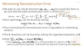
argmin
𝑾,𝒁 𝑛=1
𝑁
𝒙𝑛 − 𝑾𝒛𝑛
2 = argmin
𝑾,𝒁
𝑿 − 𝒁𝑾 2
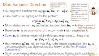
𝑤2
𝑤1
PCA is essentially doing a change of
axes in which we are representing the
data
𝑒1
𝑒2
𝑒1, 𝑒2: Standard co-ordinate axis (𝒙 = [𝑥1, 𝑥2])
𝑤1, 𝑤2: New co-ordinate axis (𝒛 = [𝑧1, 𝑧2])
Each input will still have 2 co-
ordinates, in the new co-ordinate
system, equal to the distances
measured from the new origin
To reduce dimension, can only keep the co-
ordinates of those directions that have largest
variances (e.g., in this example, if we want to
reduce to one-dim, we can keep the co-
ordinate 𝑧1 of each point along 𝑤1 and throw
away 𝑧2). We won’t lose much information Subject to
orthonormality
constraints: 𝒘𝑖
⊤
𝒘𝑗 =
0 for 𝑖 ≠ 𝑗 and 𝒘𝑖
2
=
1

6. CS771: Intro to ML
Principal Component Analysis: the algorithm
6
 Center the data (subtract the mean 𝝁 =
1
𝑁 𝑛=1
𝑁
𝒙𝑛 from each data point)
 Compute the 𝐷 × 𝐷 covariance matrix 𝐒 using the centered data matrix 𝐗 as
 Do an eigendecomposition of the covariance matrix 𝐒 (many methods exist)
 Take top 𝐾 < 𝐷 leading eigvectors {𝒘1, 𝒘2, … , 𝒘𝐾} with eigvalues
{𝜆1, 𝜆2, … , 𝜆𝐾}
 The 𝐾-dimensional projection/embedding of each input is
𝐒 =
1
𝑁
𝐗⊤
𝐗 (Assuming 𝐗 is arranged as 𝑁 × 𝐷)
𝒛𝑛 ≈ 𝐖𝐾
⊤
𝒙𝑛
𝐖K = 𝒘1, 𝒘2, … , 𝒘𝐾 is the
“projection matrix” of size
𝐷 × 𝐾
Note: Can decide how
many eigvecs to use based
on how much variance we
want to campure (recall that
each 𝜆𝑘 gives the variance
in the 𝑘𝑡ℎ
direction (and
their sum is the total
variance)

7. CS771: Intro to ML
Understanding PCA: The variance
perspective
7

8. CS771: Intro to ML
Solving PCA by Finding Max. Variance Directions
8
 Consider projecting an input 𝒙𝑛 ∈ ℝ𝐷 along a direction 𝒘1 ∈ ℝ𝐷
 Projection/embedding of 𝒙𝑛 (red points below) will be 𝒘1
⊤
𝒙𝑛 (green
pts below)
 Want 𝒘1 such that variance 𝒘1
⊤
𝑺𝒘1 is maximized
𝒘1
𝒙𝑛
Mean of projections of all inputs:
1
𝑁 𝑛=1
𝑁
𝒘1
⊤
𝒙𝑛 = 𝒘1
⊤
(
1
𝑁 𝑛=1
𝑁
𝒙𝑛) = 𝒘1
⊤
𝝁
Variance of the projections:
1
𝑁 𝑛=1
𝑁
(𝒘1
⊤
𝒙𝑛 − 𝒘1
⊤
𝝁)2 =
1
𝑁 𝑛=1
𝑁
{𝒘1
⊤
(𝒙𝑛−𝝁)}2 = 𝒘1
⊤
𝑺𝒘1
𝑺 is the 𝐷 × 𝐷 cov matrix of the
data:
𝑺 =
1
𝑁 𝑛=1
𝑁
(𝒙𝑛 − 𝝁)(𝒙𝑛 − 𝝁)⊤
For already centered data, 𝝁 = 𝟎
and 𝑺 =
1
𝑁 𝑛=1
𝑁
𝒙𝑛 𝒙𝑛
⊤
=
1
𝑁
𝑿𝑿⊤
argmax
𝒘1
𝒘1
⊤
𝑺𝒘1 s.t. 𝒘1
⊤
𝒘1 = 1
Need this constraint otherwise
the objective’s max will be

9. CS771: Intro to ML
Max. Variance Direction
9
 Our objective function was argmax
𝒘1
𝒘1
⊤
𝑺𝒘1 s.t. 𝒘1
⊤
𝒘1 = 1
 Can construct a Lagrangian for this problem
 Taking derivative w.r.t. 𝒘1 and setting to zero gives 𝑺𝒘1 = 𝜆1𝒘1
 Therefore 𝒘1 is an eigenvector of the cov matrix 𝑺 with eigenvalue 𝜆1
 Claim: 𝒘1 is the eigenvector of 𝑺 with largest eigenvalue 𝜆1. Note that
 Thus variance 𝒘1
⊤
𝑺𝒘1 will be max. if 𝜆1 is the largest eigenvalue (and 𝒘1 is
the corresponding top eigenvector; also known as the first Principal
Component)
 Other large variance directions can also be found likewise (with each being
argmax
𝒘1
𝒘1
⊤
𝑺𝒘1 + 𝜆1(1-𝒘1
⊤
𝒘1)
𝒘1
⊤
𝑺𝒘1 = 𝜆1𝒘1
⊤
𝒘1 = 𝜆1
Variance along the
direction 𝒘1
Note: In general, 𝑺
will have 𝐷 eigvecs
Note: Total variance
of the data is equal
to the sum of
eigenvalues of 𝑺, i.e.,
𝑑=1
𝐷
𝜆𝑑
PCA would keep the
top 𝐾 < 𝐷 such
directions of largest
variances

10. CS771: Intro to ML
Understanding PCA: The reconstruction
perspective
10

11. CS771: Intro to ML
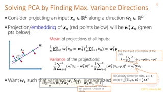
Alternate Basis and Reconstruction
11
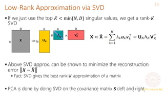
 Representing a data point 𝒙𝑛 = [𝑥𝑛1, 𝑥𝑛2, … , 𝑥𝑛𝐷] ⊤
in the standard
orthonormal basis 𝒆1, 𝒆2, … , 𝒆𝐷
 Let’s represent the same data point in a new orthonormal basis
𝒘1, 𝒘2, … , 𝒘𝐷
 Ignoring directions along which projection 𝑧𝑛𝑑 is small, we can approximate
𝒙𝑛 as
 Now 𝒙𝑛 is represented by 𝐾 < 𝐷 dim. rep. 𝒛𝑛 = [𝑧𝑛1, 𝑧𝑛2, … , 𝑧𝑛𝐾] and
(verify)
𝒙𝑛 =
𝑑=1
𝐷
𝑥𝑛𝑑𝒆𝑑
𝒆𝑑 is a vector of all zeros except a single 1
at the 𝑑𝑡ℎ
position. Also, 𝒆𝑑
⊤
𝒆𝑑′ = 0 for
𝑑 ≠ 𝑑’
𝒙𝑛 =
𝑑=1
𝐷
𝑧𝑛𝑑𝒘𝑑
𝒛𝑛 = [𝑧𝑛1, 𝑧𝑛2, … , 𝑧𝑛𝐷] ⊤
denotes
the co-ordinates of 𝒙𝑛 in the new
basis
𝑧𝑛𝑑 is the projection of 𝒙𝑛 along the
direction 𝒘𝑑 since 𝑧𝑛𝑑 = 𝒘𝑑
⊤
𝒙𝑛 =
𝒙𝑛
⊤
𝒘𝑑(verify)
𝒙𝑛 ≈ 𝒙𝑛 =
𝑑=1
𝐾
𝑧𝑛𝑑𝒘𝑑 =
𝑑=1
𝐾
(𝒙𝑛
⊤𝒘𝑑)𝒘𝑑 =
𝑑=1
𝐾
(𝒘𝑑𝒘𝑑
⊤
)𝒙𝑛
𝒛𝑛 ≈ 𝐖𝐾
⊤
𝒙𝑛
𝐖K = 𝒘1, 𝒘2, … , 𝒘𝐾 is the
“projection matrix” of size
𝐷 × 𝐾
Note that 𝒙𝑛 −
Also, 𝒙𝑛 ≈ 𝐖𝐾𝒛𝑛

12. CS771: Intro to ML
Minimizing Reconstruction Error
12
 We plan to use only 𝐾 directions 𝒘1, 𝒘2, … , 𝒘𝐾 so would like them to
be such that the total reconstruction error is minimized
 Each optimal 𝒘𝑑 can be found by solving
 Thus minimizing the reconstruction error is equivalent to maximizing
variance
 The 𝐾 directions can be found by solving the eigendecomposition of 𝐒
 Note: 𝑑=1
𝐾
𝒘𝑑
⊤
𝐒𝒘𝑑 = trace( 𝐖𝐾
⊤
𝐒𝐖𝐾)
 Thus argmax𝐖𝐾
trace( 𝑾𝐾
⊤
𝐒𝐖𝐾) s.t. orthonormality on columns of 𝐖𝑘 is the
same as solving the eigendec. of 𝑺 (recall that Spectral Clustering also required
ℒ 𝒘1, 𝒘2, … , 𝒘𝐾 =
𝑛=1
𝑁
𝒙𝑛 − 𝒙𝑛
2 =
𝑛=1
𝑁
𝒙𝑛 −
𝑑=1
𝐾
(𝒘𝑑𝒘𝑑
⊤
)𝒙𝑛
2
= 𝐶 − 𝑑=1
𝐾
𝒘𝑑
⊤
𝐒𝒘𝑑 (verify)
Constant;
doesn’t depend
on the 𝒘𝑑’s
Variance along
𝒘𝑑
argmin
𝒘𝑑
ℒ 𝒘1, 𝒘2, … , 𝒘𝐾 = argmax
𝒘𝑑
𝒘𝑑
⊤
𝐒𝒘𝑑

13. CS771: Intro to ML
Principal Component Analysis
13
 Center the data (subtract the mean 𝝁 =
1
𝑁 𝑛=1
𝑁
𝒙𝑛 from each data point)
 Compute the 𝐷 × 𝐷 covariance matrix 𝐒 using the centered data matrix 𝐗 as
 Do an eigendecomposition of the covariance matrix 𝐒 (many methods exist)
 Take top 𝐾 < 𝐷 leading eigvectors {𝒘1, 𝒘2, … , 𝒘𝐾} with eigvalues
{𝜆1, 𝜆2, … , 𝜆𝐾}
 The 𝐾-dimensional projection/embedding of each input is
𝐒 =
1
𝑁
𝐗⊤
𝐗 (Assuming 𝐗 is arranged as 𝑁 × 𝐷)
𝒛𝑛 ≈ 𝐖𝐾
⊤
𝒙𝑛
𝐖K = 𝒘1, 𝒘2, … , 𝒘𝐾 is the
“projection matrix” of size
𝐷 × 𝐾
Note: Can decide how
many eigvecs to use based
on how much variance we
want to campure (recall that
each 𝜆𝑘 gives the variance
in the 𝑘𝑡ℎ
direction (and
their sum is the total
variance)

14. CS771: Intro to ML
Singular Value Decomposition (SVD)
14
 Any matrix 𝐗 of size 𝑁 × 𝐷 can be represented as the following
decomposition
 𝐔 = 𝒖1, 𝒖2, … , 𝒖𝑁 is 𝑁 × 𝑁 matrix of left singular vectors, each 𝒖𝑛 ∈
ℝ𝑁
 𝐔 is also orthonormal
 𝐕 = 𝒗1, 𝒗2, … , 𝒗𝑁 is 𝐷 × 𝐷 matrix of right singular vectors, each 𝒗𝑑 ∈
ℝ𝐷
 𝐕 is also orthonormal
𝐗 = 𝐔𝚲𝐕⊤ =
𝑘=1
min{𝑁,𝐷}
𝜆𝑘𝒖𝑘𝒗𝑘
⊤
Diagonal matrix. If 𝑁 > 𝐷, last 𝐷 − 𝑁 rows
are all zeros; if 𝐷 > 𝑁, last 𝐷 − 𝑁 columns
are all zeros

15. CS771: Intro to ML
Low-Rank Approximation via SVD
15
 If we just use the top 𝐾 < min{𝑁, 𝐷} singular values, we get a rank-𝐾
SVD
 Above SVD approx. can be shown to minimize the reconstruction
error 𝑿 − 𝑿
 Fact: SVD gives the best rank-𝐾 approximation of a matrix
 PCA is done by doing SVD on the covariance matrix 𝐒 (left and right

16. CS771: Intro to ML
Dim-Red as Matrix Factorization
16
 If we don’t care about the orthonormality constraints, then dim-red can
also be achieved by solving a matrix factorization problem on the data
matrix 𝐗
 Can solve such problems using ALT-OPT
X Z
W
N
D D
K
K
N
≈
Matrix containing
the low-dim rep of
𝐗
𝐙, 𝐖 = argmin𝐙,𝐖 𝐗 − 𝐙𝐖 2 If 𝐾 < min{𝐷, 𝑁}, such a
factorization gives a low-rank
approximation of the data
matrix X