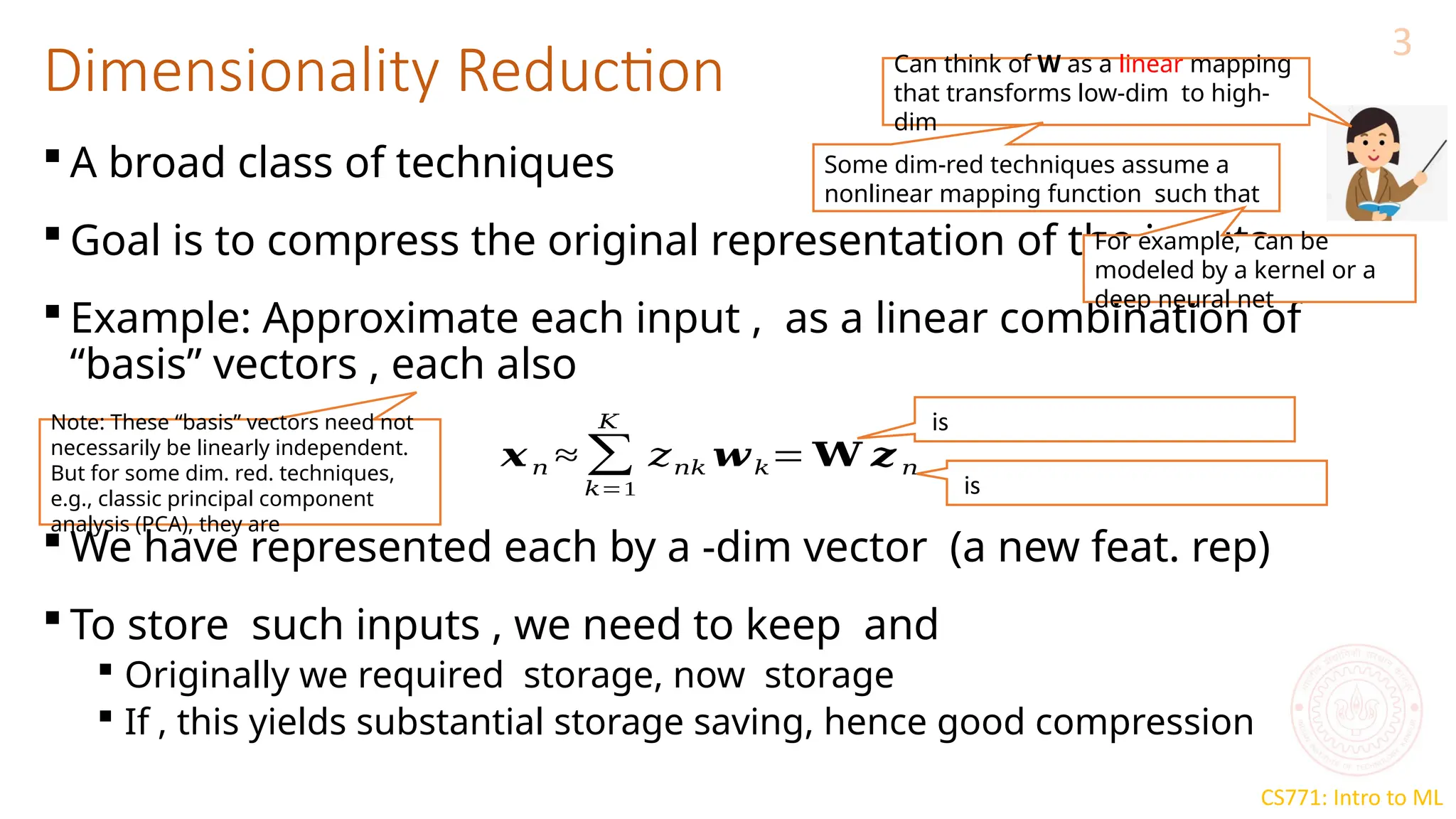
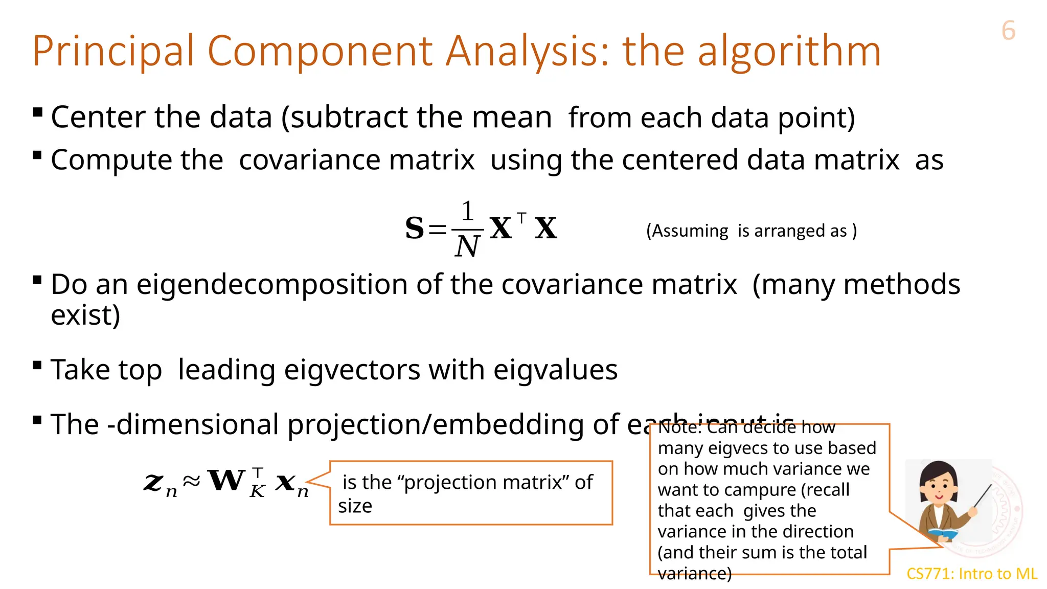
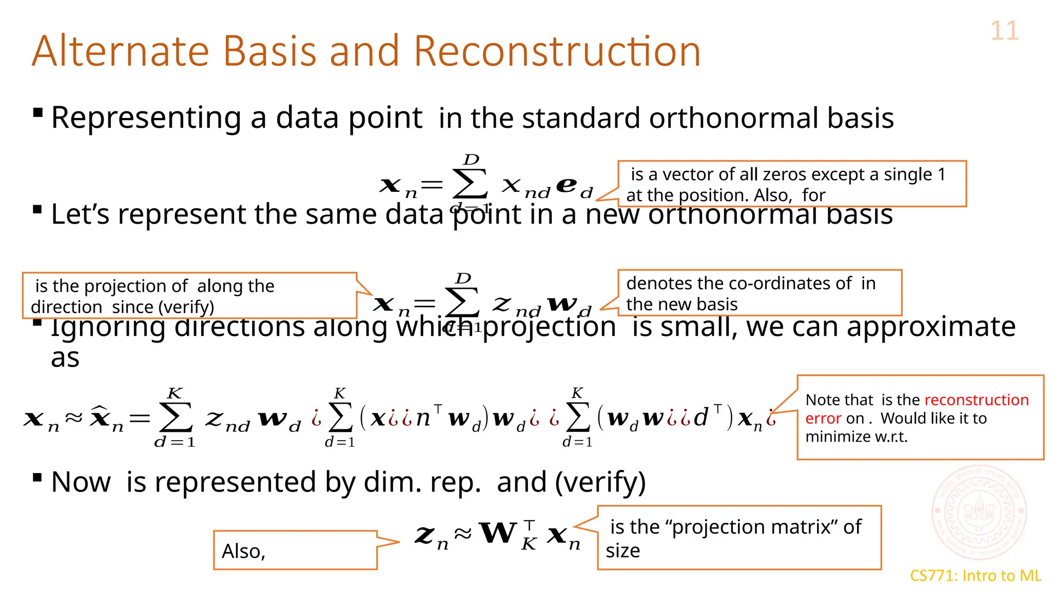
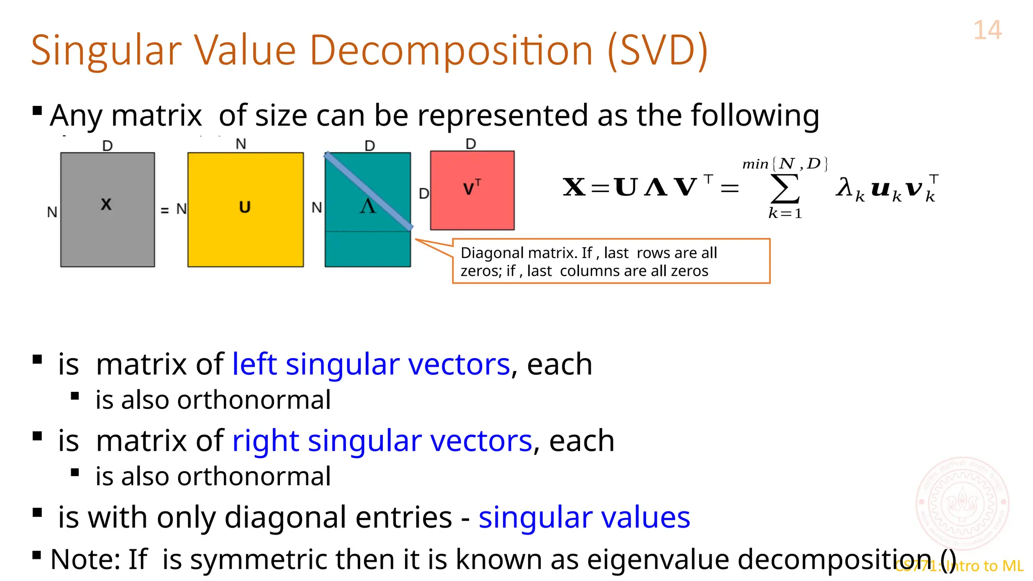
Dimensionality Reduction: Principal
Component Analysis
CS771: Introduction to Machine Learning
Nisheeth
CS771: Intro to ML
K-means loss function: recap
2
X Z
N
K
K
[, ] denotes a length
one-hot encoding of
• Remember the matrix factorization view of the k-means loss function?
• We approximated an N x D matrix with
• An NxK matrix and a
• KXD matrix
• This could be storage efficient if K is much smaller than D
D
D
CS771: Intro to ML
Dimensionality Reduction
3
 A broad class of techniques
 Goal is to compress the original representation of the inputs
 Example: Approximate each input , as a linear combination of
“basis” vectors , each also
 We have represented each by a -dim vector (a new feat. rep)
 To store such inputs , we need to keep and
 Originally we required storage, now storage
 If , this yields substantial storage saving, hence good compression
𝒙𝑛 ≈ ∑
𝑘=1
𝐾
𝑧𝑛𝑘 𝒘𝑘= 𝐖 𝒛 𝑛
is
is
Note: These “basis” vectors need not
necessarily be linearly independent.
But for some dim. red. techniques,
e.g., classic principal component
analysis (PCA), they are
Can think of W as a linear mapping
that transforms low-dim to high-
dim
Some dim-red techniques assume a
nonlinear mapping function such that
For example, can be
modeled by a kernel or a
deep neural net
CS771: Intro to ML
Dimensionality Reduction
4
 Dim-red for face images
 In this example, is a low-dim feature rep. for
 Essentially, each face image in the dataset now represented by just 4 real
numbers 
 Different dim-red algos differ in terms of how the basis vectors are
defined/learned
A face
image
K=4 “basis” face
images
Each “basis” image is like a
“template” that captures the
common properties of face
images in the dataset
𝑧𝑛 1 𝑧𝑛 2 𝑧𝑛 3 𝑧𝑛 4
𝒘1 𝒘 2 𝒘 3
𝒘 4
+
Like 4 new
features
CS771: Intro to ML
Principal Component Analysis (PCA)
5
 A classic linear dim. reduction method (Pearson, 1901; Hotelling,
1930)
 Can be seen as
 Learning directions (co-ordinate axes) that capture maximum variance in data
 Learning projection directions that result in smallest reconstruction error
arg min
𝑾 , 𝒁
∑
𝑛=1
𝑁
‖𝒙𝑛 −𝑾 𝒛𝑛‖
2
=arg min
𝑾 , 𝒁
‖𝑿 − 𝒁𝑾‖
2
𝑤2
𝑤1
PCA is essentially doing a change of
axes in which we are representing
the data
𝑒1
𝑒2
Standard co-ordinate axis ()
New co-ordinate axis ()
Each input will still have 2 co-
ordinates, in the new co-ordinate
system, equal to the distances
measured from the new origin
To reduce dimension, can only keep the co-
ordinates of those directions that have largest
variances (e.g., in this example, if we want to
reduce to one-dim, we can keep the co-
ordinate of each point along and throw away
). We won’t lose much information
Subject to
orthonormality
constraints: for and
Large variance
S
m
a
l
l
v
a
r
i
a
n
c
e
CS771: Intro to ML
Principal Component Analysis: the algorithm
6
 Center the data (subtract the mean from each data point)
 Compute the covariance matrix using the centered data matrix as
 Do an eigendecomposition of the covariance matrix (many methods
exist)
 Take top leading eigvectors with eigvalues
 The -dimensional projection/embedding of each input is
𝐒=
1
𝑁
𝐗
⊤
𝐗 (Assuming is arranged as )
𝒛𝑛 ≈ 𝐖 𝐾
⊤
𝒙𝑛 is the “projection matrix” of
size
Note: Can decide how
many eigvecs to use based
on how much variance we
want to campure (recall
that each gives the
variance in the direction
(and their sum is the total
variance)
CS771: Intro to ML
Understanding PCA: The variance perspective
7
CS771: Intro to ML
Solving PCA by Finding Max. Variance Directions
8
 Consider projecting an input along a direction
 Projection/embedding of (red points below) will be (green pts
below)
 Want such that variance is maximized
𝒘1
𝒙𝑛
𝒘 1
⊤ 𝒙 𝑛
Mean of projections of all inputs:
Variance of the projections:
is the cov matrix of the data:
For already centered data, = and
=
s.t.
Need this constraint otherwise
the objective’s max will be
CS771: Intro to ML
Max. Variance Direction
9
 Our objective function was s.t.
 Can construct a Lagrangian for this problem
 Taking derivative w.r.t. and setting to zero gives
 Therefore is an eigenvector of the cov matrix with eigenvalue
 Claim: is the eigenvector of with largest eigenvalue . Note that
 Thus variance will be max. if is the largest eigenvalue (and is the
corresponding top eigenvector; also known as the first Principal
Component)
 Other large variance directions can also be found likewise (with each
1-
Variance along
the direction
Note: In general,
will have eigvecs
Note: Total variance
of the data is equal
to the sum of
eigenvalues of , i.e.,
PCA would keep the
top such directions
of largest variances
CS771: Intro to ML
Understanding PCA: The reconstruction perspective
10
CS771: Intro to ML
Alternate Basis and Reconstruction
11
 Representing a data point in the standard orthonormal basis
 Let’s represent the same data point in a new orthonormal basis
 Ignoring directions along which projection is small, we can approximate
as
 Now is represented by dim. rep. and (verify)
𝒙𝑛=∑
𝑑=1
𝐷
𝑥𝑛𝑑 𝒆𝑑
is a vector of all zeros except a single 1
at the position. Also, for
𝒙𝑛=∑
𝑑=1
𝐷
𝑧 𝑛𝑑 𝒘𝑑
denotes the co-ordinates of in
the new basis
is the projection of along the
direction since (verify)
𝒙𝑛 ≈ ^
𝒙𝑛=∑
𝑑=1
𝐾
𝑧𝑛𝑑 𝒘𝑑 ¿ ∑
𝑑=1
𝐾
( 𝒙¿¿𝑛⊤
𝒘𝑑)𝒘𝑑 ¿ ¿ ∑
𝑑=1
𝐾
(𝒘𝑑 𝒘¿¿𝑑
⊤
) 𝒙𝑛 ¿
𝒛𝑛 ≈ 𝐖 𝐾
⊤
𝒙𝑛
is the “projection matrix” of
size
Note that is the reconstruction
error on . Would like it to
minimize w.r.t.
Also,
CS771: Intro to ML
Minimizing Reconstruction Error
12
 We plan to use only directions so would like them to be such that
the total reconstruction error is minimized
 Each optimal can be found by solving
 Thus minimizing the reconstruction error is equivalent to
maximizing variance
 The directions can be found by solving the eigendecomposition of
 Note:
 Thus s.t. orthonormality on columns of is the same as solving the
eigendec. of (recall that Spectral Clustering also required solving this)
ℒ ( 𝒘1 , 𝒘2 , … , 𝒘 𝐾 )=∑
𝑛=1
𝑁
‖𝒙 𝑛 − ^
𝒙 𝑛‖
2
=∑
𝑛=1
𝑁
¿ ¿ ¿ ¿ (verify)
Constant; doesn’t
depend on the ’s
Variance along
CS771: Intro to ML
Principal Component Analysis
13
 Center the data (subtract the mean from each data point)
 Compute the covariance matrix using the centered data matrix as
 Do an eigendecomposition of the covariance matrix (many methods
exist)
 Take top leading eigvectors with eigvalues
 The -dimensional projection/embedding of each input is
𝐒=
1
𝑁
𝐗
⊤
𝐗 (Assuming is arranged as )
𝒛𝑛 ≈ 𝐖 𝐾
⊤
𝒙𝑛 is the “projection matrix” of
size
Note: Can decide how
many eigvecs to use based
on how much variance we
want to campure (recall
that each gives the
variance in the direction
(and their sum is the total
variance)
CS771: Intro to ML
Singular Value Decomposition (SVD)
14
 Any matrix of size can be represented as the following
decomposition
 is matrix of left singular vectors, each
 is also orthonormal
 is matrix of right singular vectors, each
 is also orthonormal
 is with only diagonal entries - singular values
 Note: If is symmetric then it is known as eigenvalue decomposition ()
𝐗=𝐔 𝚲 𝐕⊤
= ∑
𝑘=1
min {𝑁 , 𝐷 }
𝜆𝑘 𝒖𝑘 𝒗𝑘
⊤
Diagonal matrix. If , last rows are all
zeros; if , last columns are all zeros
CS771: Intro to ML
Low-Rank Approximation via SVD
15
 If we just use the top singular values, we get a rank- SVD
 Above SVD approx. can be shown to minimize the reconstruction
error
 Fact: SVD gives the best rank- approximation of a matrix
 PCA is done by doing SVD on the covariance matrix (left and right
singular vectors are the same and become eigenvectors, singular values
CS771: Intro to ML
Dim-Red as Matrix Factorization
16
 If we don’t care about the orthonormality constraints, then dim-red can
also be achieved by solving a matrix factorization problem on the data
matrix
 Can solve such problems using ALT-OPT
X Z
W
N
D D
K
K
N
≈
Matrix containing
the low-dim rep of
{^
𝐙 , ^
𝐖 }=argmin𝐙, 𝐖 ‖𝐗 −𝐙𝐖‖
2
If , such a factorization gives a
low-rank approximation of the
data matrix X

lec22 pca- DIMENSILANITY REDUCTION.pptx

  • 1.
    Dimensionality Reduction: Principal ComponentAnalysis CS771: Introduction to Machine Learning Nisheeth
  • 2.
    CS771: Intro toML K-means loss function: recap 2 X Z N K K [, ] denotes a length one-hot encoding of • Remember the matrix factorization view of the k-means loss function? • We approximated an N x D matrix with • An NxK matrix and a • KXD matrix • This could be storage efficient if K is much smaller than D D D
  • 3.
    CS771: Intro toML Dimensionality Reduction 3  A broad class of techniques  Goal is to compress the original representation of the inputs  Example: Approximate each input , as a linear combination of “basis” vectors , each also  We have represented each by a -dim vector (a new feat. rep)  To store such inputs , we need to keep and  Originally we required storage, now storage  If , this yields substantial storage saving, hence good compression 𝒙𝑛 ≈ ∑ 𝑘=1 𝐾 𝑧𝑛𝑘 𝒘𝑘= 𝐖 𝒛 𝑛 is is Note: These “basis” vectors need not necessarily be linearly independent. But for some dim. red. techniques, e.g., classic principal component analysis (PCA), they are Can think of W as a linear mapping that transforms low-dim to high- dim Some dim-red techniques assume a nonlinear mapping function such that For example, can be modeled by a kernel or a deep neural net
  • 4.
    CS771: Intro toML Dimensionality Reduction 4  Dim-red for face images  In this example, is a low-dim feature rep. for  Essentially, each face image in the dataset now represented by just 4 real numbers   Different dim-red algos differ in terms of how the basis vectors are defined/learned A face image K=4 “basis” face images Each “basis” image is like a “template” that captures the common properties of face images in the dataset 𝑧𝑛 1 𝑧𝑛 2 𝑧𝑛 3 𝑧𝑛 4 𝒘1 𝒘 2 𝒘 3 𝒘 4 + Like 4 new features
  • 5.
    CS771: Intro toML Principal Component Analysis (PCA) 5  A classic linear dim. reduction method (Pearson, 1901; Hotelling, 1930)  Can be seen as  Learning directions (co-ordinate axes) that capture maximum variance in data  Learning projection directions that result in smallest reconstruction error arg min 𝑾 , 𝒁 ∑ 𝑛=1 𝑁 ‖𝒙𝑛 −𝑾 𝒛𝑛‖ 2 =arg min 𝑾 , 𝒁 ‖𝑿 − 𝒁𝑾‖ 2 𝑤2 𝑤1 PCA is essentially doing a change of axes in which we are representing the data 𝑒1 𝑒2 Standard co-ordinate axis () New co-ordinate axis () Each input will still have 2 co- ordinates, in the new co-ordinate system, equal to the distances measured from the new origin To reduce dimension, can only keep the co- ordinates of those directions that have largest variances (e.g., in this example, if we want to reduce to one-dim, we can keep the co- ordinate of each point along and throw away ). We won’t lose much information Subject to orthonormality constraints: for and Large variance S m a l l v a r i a n c e
  • 6.
    CS771: Intro toML Principal Component Analysis: the algorithm 6  Center the data (subtract the mean from each data point)  Compute the covariance matrix using the centered data matrix as  Do an eigendecomposition of the covariance matrix (many methods exist)  Take top leading eigvectors with eigvalues  The -dimensional projection/embedding of each input is 𝐒= 1 𝑁 𝐗 ⊤ 𝐗 (Assuming is arranged as ) 𝒛𝑛 ≈ 𝐖 𝐾 ⊤ 𝒙𝑛 is the “projection matrix” of size Note: Can decide how many eigvecs to use based on how much variance we want to campure (recall that each gives the variance in the direction (and their sum is the total variance)
  • 7.
    CS771: Intro toML Understanding PCA: The variance perspective 7
  • 8.
    CS771: Intro toML Solving PCA by Finding Max. Variance Directions 8  Consider projecting an input along a direction  Projection/embedding of (red points below) will be (green pts below)  Want such that variance is maximized 𝒘1 𝒙𝑛 𝒘 1 ⊤ 𝒙 𝑛 Mean of projections of all inputs: Variance of the projections: is the cov matrix of the data: For already centered data, = and = s.t. Need this constraint otherwise the objective’s max will be
  • 9.
    CS771: Intro toML Max. Variance Direction 9  Our objective function was s.t.  Can construct a Lagrangian for this problem  Taking derivative w.r.t. and setting to zero gives  Therefore is an eigenvector of the cov matrix with eigenvalue  Claim: is the eigenvector of with largest eigenvalue . Note that  Thus variance will be max. if is the largest eigenvalue (and is the corresponding top eigenvector; also known as the first Principal Component)  Other large variance directions can also be found likewise (with each 1- Variance along the direction Note: In general, will have eigvecs Note: Total variance of the data is equal to the sum of eigenvalues of , i.e., PCA would keep the top such directions of largest variances
  • 10.
    CS771: Intro toML Understanding PCA: The reconstruction perspective 10
  • 11.
    CS771: Intro toML Alternate Basis and Reconstruction 11  Representing a data point in the standard orthonormal basis  Let’s represent the same data point in a new orthonormal basis  Ignoring directions along which projection is small, we can approximate as  Now is represented by dim. rep. and (verify) 𝒙𝑛=∑ 𝑑=1 𝐷 𝑥𝑛𝑑 𝒆𝑑 is a vector of all zeros except a single 1 at the position. Also, for 𝒙𝑛=∑ 𝑑=1 𝐷 𝑧 𝑛𝑑 𝒘𝑑 denotes the co-ordinates of in the new basis is the projection of along the direction since (verify) 𝒙𝑛 ≈ ^ 𝒙𝑛=∑ 𝑑=1 𝐾 𝑧𝑛𝑑 𝒘𝑑 ¿ ∑ 𝑑=1 𝐾 ( 𝒙¿¿𝑛⊤ 𝒘𝑑)𝒘𝑑 ¿ ¿ ∑ 𝑑=1 𝐾 (𝒘𝑑 𝒘¿¿𝑑 ⊤ ) 𝒙𝑛 ¿ 𝒛𝑛 ≈ 𝐖 𝐾 ⊤ 𝒙𝑛 is the “projection matrix” of size Note that is the reconstruction error on . Would like it to minimize w.r.t. Also,
  • 12.
    CS771: Intro toML Minimizing Reconstruction Error 12  We plan to use only directions so would like them to be such that the total reconstruction error is minimized  Each optimal can be found by solving  Thus minimizing the reconstruction error is equivalent to maximizing variance  The directions can be found by solving the eigendecomposition of  Note:  Thus s.t. orthonormality on columns of is the same as solving the eigendec. of (recall that Spectral Clustering also required solving this) ℒ ( 𝒘1 , 𝒘2 , … , 𝒘 𝐾 )=∑ 𝑛=1 𝑁 ‖𝒙 𝑛 − ^ 𝒙 𝑛‖ 2 =∑ 𝑛=1 𝑁 ¿ ¿ ¿ ¿ (verify) Constant; doesn’t depend on the ’s Variance along
  • 13.
    CS771: Intro toML Principal Component Analysis 13  Center the data (subtract the mean from each data point)  Compute the covariance matrix using the centered data matrix as  Do an eigendecomposition of the covariance matrix (many methods exist)  Take top leading eigvectors with eigvalues  The -dimensional projection/embedding of each input is 𝐒= 1 𝑁 𝐗 ⊤ 𝐗 (Assuming is arranged as ) 𝒛𝑛 ≈ 𝐖 𝐾 ⊤ 𝒙𝑛 is the “projection matrix” of size Note: Can decide how many eigvecs to use based on how much variance we want to campure (recall that each gives the variance in the direction (and their sum is the total variance)
  • 14.
    CS771: Intro toML Singular Value Decomposition (SVD) 14  Any matrix of size can be represented as the following decomposition  is matrix of left singular vectors, each  is also orthonormal  is matrix of right singular vectors, each  is also orthonormal  is with only diagonal entries - singular values  Note: If is symmetric then it is known as eigenvalue decomposition () 𝐗=𝐔 𝚲 𝐕⊤ = ∑ 𝑘=1 min {𝑁 , 𝐷 } 𝜆𝑘 𝒖𝑘 𝒗𝑘 ⊤ Diagonal matrix. If , last rows are all zeros; if , last columns are all zeros
  • 15.
    CS771: Intro toML Low-Rank Approximation via SVD 15  If we just use the top singular values, we get a rank- SVD  Above SVD approx. can be shown to minimize the reconstruction error  Fact: SVD gives the best rank- approximation of a matrix  PCA is done by doing SVD on the covariance matrix (left and right singular vectors are the same and become eigenvectors, singular values
  • 16.
    CS771: Intro toML Dim-Red as Matrix Factorization 16  If we don’t care about the orthonormality constraints, then dim-red can also be achieved by solving a matrix factorization problem on the data matrix  Can solve such problems using ALT-OPT X Z W N D D K K N ≈ Matrix containing the low-dim rep of {^ 𝐙 , ^ 𝐖 }=argmin𝐙, 𝐖 ‖𝐗 −𝐙𝐖‖ 2 If , such a factorization gives a low-rank approximation of the data matrix X